options(java.parameters = "-Xmx2G")![]() In this first hands-on section of the workshop, we’ll learn a very quick and simple way to calculate spatial accessibility using the
In this first hands-on section of the workshop, we’ll learn a very quick and simple way to calculate spatial accessibility using the {r5r} package. In the next section, we’ll see a more flexible and robust way to do the same thing. Here we’ll be calculating the number of schools accessible by public transport within a travel time of 20 minutes.
1. Allocating memory to Java & loading packages
First, let’s increase the memory available to run Java, which is used by the underlying R5 routing engine. To increase the available memory to 2 GB, for example, we use the following command. Note that this needs to be run before loading the packages that will be used in our analysis.
Now we can load the packages we’ll use in this section:
library(r5r)
library(h3jsr)
library(dplyr)
library(mapview)
library(ggplot2)
2. A quick look at our sample data
Our case study is the city of Porto Alegre, Brazil. The {r5r} package brings a small sample data for this city, including the following files:
- An OpenStreetMap network:
poa_osm.pbf - Two public transport GTFS feeds:
poa_eptc.zip(buses) andpoa_trensurb.zip(trains) - A raster elevation data:
poa_elevation.tif - A data frame with land use data:
poa_hexgrid.csvfile with the centroids of a regular hexagonal grid covering the sample area. The data frame also indicates the number of residents and schools in each cell. We’ll use these points as origins and destinations in our analysis.
These data sets should be saved in a single directory (our data_path). Here’s how the land use data looks like:
# path to data directory
data_path <- system.file("extdata/poa", package = "r5r")

# read points data
points <- read.csv(file.path(data_path, "poa_hexgrid.csv"))
head(points)
id lon lat population schools jobs healthcare
1 89a901291abffff -51.15825 -30.05385 0 0 1214 0
2 89a9012a3cfffff -51.21187 -30.10058 159 0 0 0
3 89a901295b7ffff -51.16521 -30.07544 1008 0 3 1
4 89a901284a3ffff -51.20535 -30.09005 92 0 0 0
5 89a9012809bffff -51.19575 -30.07839 577 0 9 0
6 89a901285cfffff -51.21108 -30.08124 1170 0 427 0🔎 To visualize the spatial distribution of these data, we can retrieve the geometry of the H3 hexagonal grid and explore it using an interactive map:
# retrieve polygons of H3 spatial grid
grid <- h3jsr::cell_to_polygon(
  points$id,
  simple = FALSE
  )

# merge spatial grid with land use data
grid_poa <- left_join(
  grid,
  points,
  by = c('h3_address'='id')
  )

# interactive map
mapview(grid_poa, zcol = 'population')
3. Building a routable transport network
This quick approach to calculate accessibility involves only 2 steps. The first step is to build the multimodal transport network using the r5r::setup_r5() function.
r5r_core <- r5r::setup_r5(data_path,
                          verbose = FALSE)
As you can see, we only need to pass the path to our data directory to the r5r::setup_r5() function. The function then combines the OSM, GTFS and elevation data in this directory to create a graph that is used for routing trips between origin-destination pairs and, consequently, for calculating travel time matrices and accessibility.
4. Calculating access: quick approach
In the second step, you can calculate accessibility estimates in a single call using the r5r::accessibility() function. It includes different options of decay functions to compute cumulative accessibility measures and different gravity-based metrics.
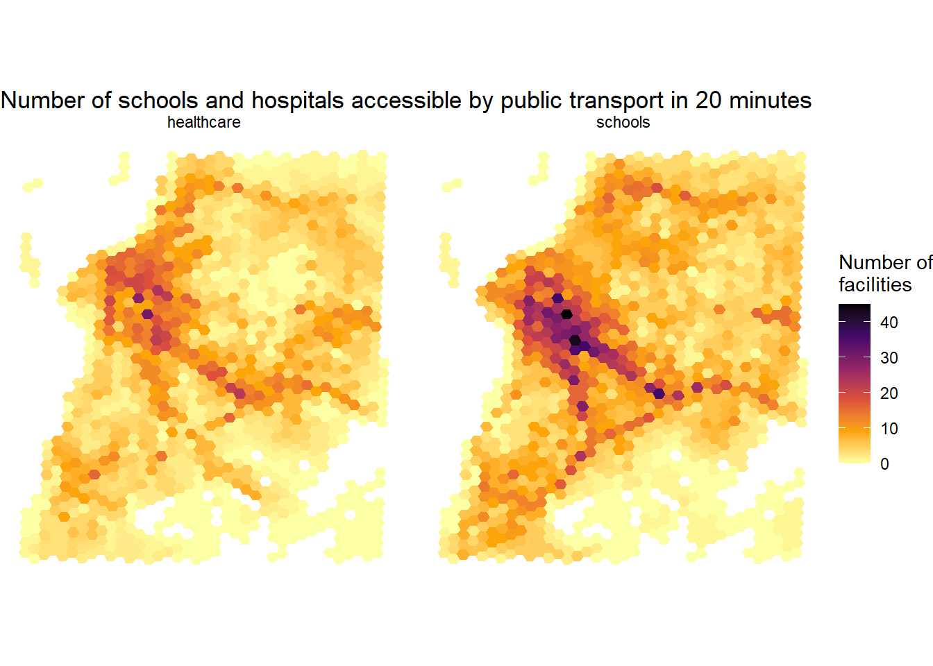
In this example, we calculate the cumulative accessibility of the number of schools and hospitals accessible in less than 20 minutes by public transport. Thus, we’ll be using decay_function = "step".
Note that to use r5r::accessibility(), the input of points must be a data.frame with columns indicating:
- the
idof each location - spatial coordinates
latandlon - the number of activities in each location. The name of this column has to be passed to the
opportunities_colnamesparameter.
# routing inputs
mode <- c("walk", "transit")
max_walk_time <- 30
travel_time_cutoff <- 20
departure_datetime <- as.POSIXct("13-05-2019 14:00:00",
format = "%d-%m-%Y %H:%M:%S")
# calculate accessibility
access1 <- r5r::accessibility(
r5r_core = r5r_core,
origins = points,
destinations = points,
mode = mode,
opportunities_colnames = c("schools", "healthcare"),
decay_function = "step",
cutoffs = travel_time_cutoff,
departure_datetime = departure_datetime,
max_walk_time = max_walk_time,
progress = TRUE
)- 1
- In minutes
- 2
- Note you can pass the columns of more than one type of opportunity.
- 3
- Similarly, you could pass more than one time threshold.
Tip
Note that the r5r::accessibility() function has several additional parameters that allow you to specify different characteristics of trips, including a maximum trip duration, walking and cycling speed, level of traffic stress (LTS), etc. For more info, check the documentation of the function by calling ?r5r::accessibility in your R Console or check the documentation on {r5r} website.
The output is a data.frame that shows for every origin id the number of opportunities that can be reached:
head(access1) id opportunity percentile cutoff accessibility
<char> <char> <int> <int> <num>
1: 89a901291abffff schools 50 20 3
2: 89a901291abffff healthcare 50 20 6
3: 89a9012a3cfffff schools 50 20 0
4: 89a9012a3cfffff healthcare 50 20 0
5: 89a901295b7ffff schools 50 20 6
6: 89a901295b7ffff healthcare 50 20 45. Accessibility map
Now it is super simple to merge these accessibility estimates to our spatial grid to visualize these results on a map.
# merge spatial grid with accessibility estimates
access_sf <- left_join(
  grid,
  access1,
  by = c('h3_address'='id')
  )

# plot
ggplot() +
  geom_sf(data = access_sf, aes(fill = accessibility), color= NA) +
  scale_fill_viridis_c(direction = -1, option = 'B') +
  labs(title = 'Number of schools and hospitals accessible by public transport in 20 minutes',
       fill = 'Number of\nfacilities') +
  theme_minimal() +
  theme(axis.title = element_blank()) +
  facet_wrap(~opportunity) +
  theme_void()