Exploring Emission Factors

Emission factor models tell us the mass of pollutants that are expected to be emitted by a given vehicle given a few characteristics such as vehicle age, type, fuel, technology, speed, and distance traveled. Various environmental agencies develop these functional relations based on data collected from local measurements. Understanding how emission factor data work is very important to understand how the emission estimates of a given vehicle or public transport system are influenced by the methodological choices of which emission factor model should be used. This vignette helps users explore the emission factors data available in the gtfs2emis package.

Available emission factor models

The gtfs2emis package currently includes hot-exhaust emission factor data from four environmental agencies. Reports with detailed information and methods on how these emission factor data were originally calculated can be found on the agencies’ websites in the links below

Hot-exhaust emissions

- Brazil, Environment Company of Sao Paulo — CETESB

- United States, Environmental Protection Agency — MOVES3 Model

- United States, California Air Resources Board — EMFAC2017 model

- Europe, European Environment Agency — EMEP-EEA

Wear emissions (tire, brake and road wear)

- Europe, European Environment Agency — EMEP-EEA

Visualizing emission factor data

Emission fator values vary by fleet characteristics — as shown in Defining Fleet data vignette. In this section we will use the ef_europe_emep() function and look at three types of urban buses (Midi, Standard and Articulated) to illustrate how emissions vary according to vehicle type, average speed, and pollutant.

#library(gtfs2emis)

library(units)
library(gtfs2emis)
library(ggplot2)


ef_europe <- ef_europe_emep(speed = units::set_units(10:100,"km/h")
                            ,veh_type = c("Ubus Midi <=15 t"
                                          ,"Ubus Std 15 - 18 t"
                                          ,"Ubus Artic >18 t")
                            ,euro = c("III", "IV", "V")
                            ,pollutant = c("PM10", "NOx")
                            ,fuel = c("D", "D", "D")
                            ,tech = c("-", "SCR", "SCR")
                            ,as_list = TRUE)
names(ef_europe)
#>  [1] "pollutant" "veh_type"  "euro"      "fuel"      "tech"      "process"  
#>  [7] "slope"     "load"      "speed"     "EF"

In the case above, the function returns a list that contains all the relevant information for the emission factor — shown in names(ef_europe). However, it may be useful to check the emission factor results in a data.frame or graphic format.

ef_europe_dt <- emis_to_dt(emi_list = ef_europe
                           ,emi_vars = "EF"
                           ,veh_vars = c("veh_type","euro","fuel","tech")
                           ,pol_vars = "pollutant"
                           ,segment_vars = c("slope","load","speed"))
head(ef_europe_dt)
#>            veh_type   euro   fuel   tech pollutant               EF     process
#>              <char> <char> <char> <char>    <char>          <units>      <char>
#> 1: Ubus Midi <=15 t    III      D      -      PM10 0.2559070 [g/km] hot_exhaust
#> 2: Ubus Midi <=15 t    III      D      -      PM10 0.2559070 [g/km] hot_exhaust
#> 3: Ubus Midi <=15 t    III      D      -      PM10 0.2413421 [g/km] hot_exhaust
#> 4: Ubus Midi <=15 t    III      D      -      PM10 0.2285624 [g/km] hot_exhaust
#> 5: Ubus Midi <=15 t    III      D      -      PM10 0.2172637 [g/km] hot_exhaust
#> 6: Ubus Midi <=15 t    III      D      -      PM10 0.2072074 [g/km] hot_exhaust
#>    slope  load     speed
#>    <num> <num>   <units>
#> 1:     0   0.5 10 [km/h]
#> 2:     0   0.5 11 [km/h]
#> 3:     0   0.5 12 [km/h]
#> 4:     0   0.5 13 [km/h]
#> 5:     0   0.5 14 [km/h]
#> 6:     0   0.5 15 [km/h]

Plotting the speed-dependent emission factors according to vehicle type (veh_type) and euro standard (euro).

ef_europe_dt$name_fleet <- paste(ef_europe_dt$veh_type, "/ Euro"
                                 , ef_europe_dt$euro)

# plot
ggplot(ef_europe_dt) + 
  geom_line(aes(x = speed,y = EF,color = name_fleet))+
  labs(color = "Category / EURO")+
  facet_wrap(~pollutant,scales = "free")+
  theme(legend.position = "bottom")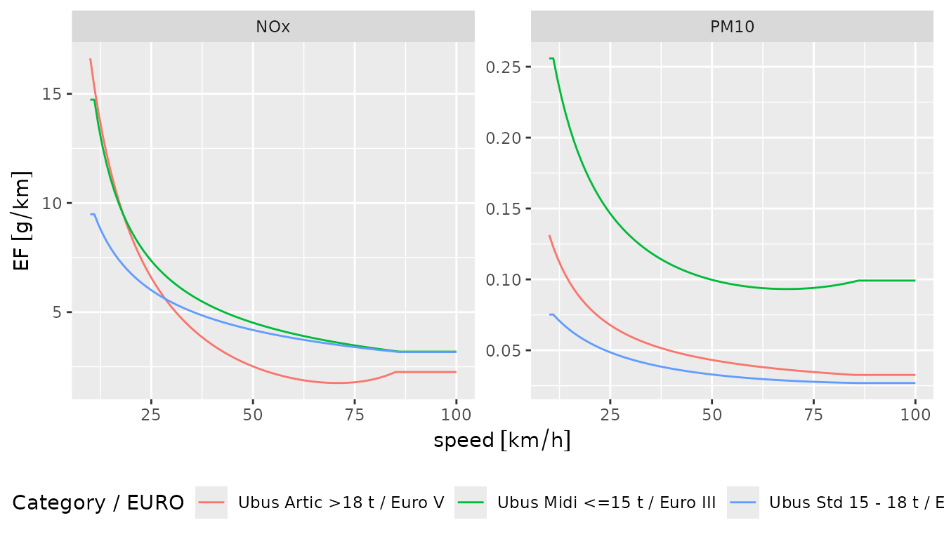
#> Warning: The `scale_name` argument of `continuous_scale()` is deprecated as of ggplot2
#> 3.5.0.
#> This warning is displayed once every 8 hours.
#> Call `lifecycle::last_lifecycle_warnings()` to see where this warning was
#> generated.

There are situations where the emission factor are not available for a given input parameter. In the case of ef_europe_emep() function, when the information on vehicle technology does not match the existing database, the package displays a message indicating the technology considered. Please check the message shown in the code block below. In such case, users can either select existing data for the combining variables (euro, tech, veh_type, and pollutant), or accept the assumed change in vehicle technology.

ef_europe_co2 <- ef_europe_emep(speed = units::set_units(10:100,"km/h")
                                ,veh_type = "Ubus Std 15 - 18 t"
                                ,euro = "VI",pollutant = "CO2"
                                ,tech = "DPF+SCR"
                                ,as_list = TRUE)
#> 'CO2' Emission factor not found for 'DPF+SCR' Technology and Euro 'VI'.
#>  The package assumed 'SCR' Technology entry. Please check `data(ef_europe_emep_db)` for available data.

The other EF functions, ef_usa_emfac(), ef_usa_moves() and ef_brazil_cetesb() work in a similar way. See the functions documentation for more detail.

Scaling Emission Factors: making emission factors speed-dependent

For most models (MOVES3, EMEP-EEA and EMFAC2017), emission factors depend on a vehicle’s speed. However, the emission factors developed for Brazil by CETESB (ef_brazil_cetesb()) do not vary by vehicle speed. In such a case, users can “scale” or adjust the local emission factor values to make them speed-dependent using the function ef_scaled_euro().

When using the EMEP-EEA model as a reference, the scaled emission factor varies according to vehicle’s speed following the expression:

$EF_{scaled} (V) = EF_{local} * \frac{EF_{euro}(V)}{EF_{euro}(SDC)},$ where $EF_{scaled}(V)$ is the scaled emission factor for each street link, $EF_{local}$ is the local emission factor, $EF_{euro}(V)$ and $EF_{euro}(SDC)$ are the EMEP/EEA emission factor the speed of V and the average urban driving speed SDC, respectively.

The scaled behavior of EF can be verified graphically when we plot the $EF_{local}$ , $EF_{scaled}(V)$ , and the $EF_{euro}(V)$ that is used as the reference To plot these data, we need six quick steps:

Build a data.frame of fleet indicating the correspondence between the fleet characteristic in the local and European emission models

fleet_filepath <- system.file("extdata/bra_cur_fleet.txt", package = "gtfs2emis")
cur_fleet <- read.table(fleet_filepath,header = TRUE, sep = ",", nrows = 1)
cur_fleet
#>   year euro shape_id type_name_br           veh_type total fuel
#> 1 2006  III     1849  BUS_URBAN_D Ubus Std 15 - 18 t     2    D

Estimate local emission factors

cur_local_ef <- ef_brazil_cetesb(pollutant = "CO2"
                                 ,veh_type = cur_fleet$type_name_br
                                 ,model_year = cur_fleet$year)
head(cur_local_ef)
#> $pollutant
#> [1] "CO2"
#> 
#> $veh_type
#> [1] "BUS_URBAN_D"
#> 
#> $model_year
#> [1] 2006
#> 
#> $EF
#> Units: [g/km]
#>      CO2_2006
#> [1,] 1385.626
#> 
#> $process
#> [1] "hot_exhaust"

# convert Local EF to data.frame
cur_local_ef_dt <- emis_to_dt(emi_list = cur_local_ef
                             ,emi_vars = "EF")

Estimate ef_emep_europe

# Euro EF
cur_euro_ef <- ef_europe_emep(speed = units::set_units(10:100,"km/h")
                              ,veh_type = cur_fleet$veh_type
                              ,euro = cur_fleet$euro
                              ,pollutant = "CO2"
                              ,tech = "-"
)

# convert to data.frame
cur_euro_ef_dt <- emis_to_dt(emi_list = cur_euro_ef
                             ,emi_vars = "EF"
                             ,veh_vars = c("veh_type","euro","fuel","tech")
                             ,segment_vars = "speed")
cur_euro_ef_dt$source <- "Euro EF"

Apply ef_scaled_euro()

cur_scaled_ef <- ef_scaled_euro(ef_local = cur_local_ef$EF
                                ,speed = units::set_units(10:100,"km/h")
                                ,veh_type = cur_fleet$veh_type
                                ,euro = cur_fleet$euro
                                ,pollutant = "CO2"
                                ,tech = "-"
                                )
# convert to data.frame
cur_scaled_ef_dt <- emis_to_dt(emi_list = cur_scaled_ef
                               ,emi_vars = "EF"
                               ,veh_vars = c("veh_type","euro","fuel","tech")
                               ,segment_vars = "speed")
cur_scaled_ef_dt$source <- "Scaled EF"

View in ggplot2

# rbind data
cur_ef <- rbind(cur_euro_ef_dt, cur_scaled_ef_dt)
cur_ef$source <- factor(cur_ef$source
                        ,levels = c("Scaled EF", "Euro EF"))

# plot
ggplot() + 
  # add scaled and euro EF
  geom_line(data = cur_ef
            ,aes(x = speed,y = EF
                 ,group = source,color = source))+
  # add local EF
  geom_hline(aes(yintercept = cur_local_ef_dt$EF)
            ,colour = "black",linetype="dashed") + 
  geom_point(aes(x = units::set_units(19,'km/h')
                 ,y = cur_local_ef$EF)) + 
  # add local EF text
  geom_text(aes(x = units::set_units(19,'km/h')
                , y = cur_local_ef_dt$EF)
            ,label = sprintf('Local EF = %s g/km at 19 km/h',round(cur_local_ef_dt$EF,1))
            ,hjust = 0,nudge_y = 100,nudge_x = 1
            ,size = 3,fontface = 1)+
  # configs plots
  scale_color_manual(values=c("red","blue"))+
  coord_cartesian(ylim = c(0,max(cur_scaled_ef_dt$EF)))+
  labs(color = NULL)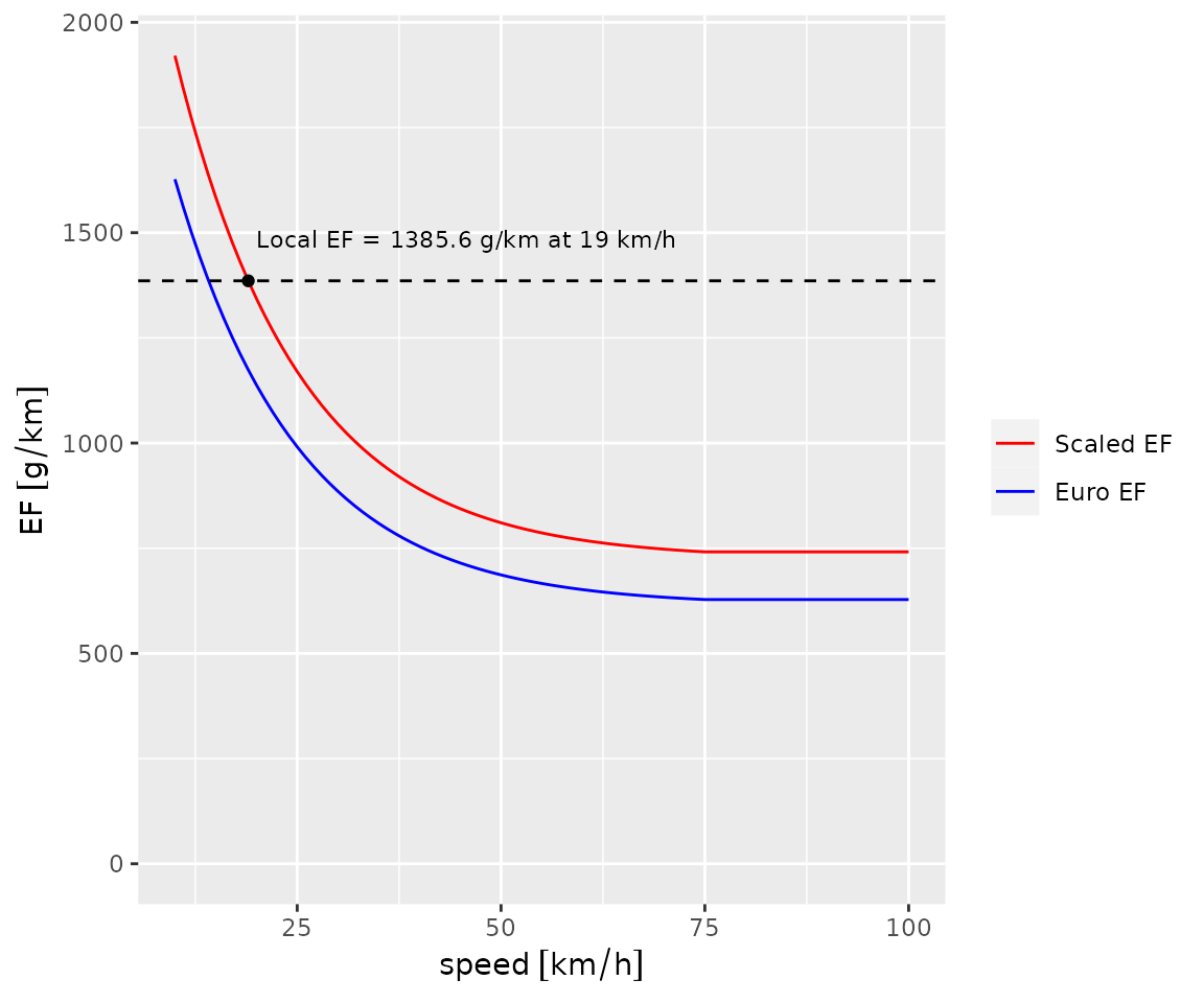

In this case, the scaled_EF has the same value of local_EF (dashed line) when speed = 19 km/h, and a similar decaying behavior as Euro_EF as speed decreases.

Checking `gtfs2emis` imported data

Users can have a closer look to the hot-exhaust emission factor data included in the package by using the following functions:

data(ef_brazil_cetesb) from Environment Company of Sao Paulo, Brazil (CETESB)
data(ef_usa_moves) from MOtor Vehicle Emission Simulator (MOVES)
data(ef_usa_emfac) from California Air Resources Board (EMFAC Model)
data(ef_europe_emep) from European Environment Agency (EMEP/EEA)

The data presented on the agencies website and software was downloaded and pre-processed in gtfs2emis to be easily read by the emission factor functions. Users can also access the scripts used to process raw data in the gtfs2emis GitHub repository.

Learn more

Check out our extra guides:

Exploring Non-Exhaust Emission Factors

Report a bug

If you have any suggestions or want to report an error, please visit the package GitHub page.