
Getting started
2026-02-12
Source:vignettes/gtfs2emis_intro_vignette.Rmd
gtfs2emis_intro_vignette.RmdAbstract
gtfs2emis is an R package to estimate public
transport emissions using data in the General Transit Feed
Specification (GTFS) format. The package allows users to estimate
the emission levels of several types of pollutants for each public
transport vehicle/trip/route at high spatial and temporal
resolutions simply using a GTFS feed and some information on fleet
characteristics.
1. Introduction
gtfs2emis is an R package to estimate hot exhaust
emissions of public transport vehicles using data in the General Transit
Feed Specification (GTFS) format. The package allows users to estimate
the emission levels of several types of pollutants for each public
transport vehicle/trip/route at high spatial and temporal resolutions
simply using a GTFS feed and some information on fleet characteristics.
This vignette introduces the main functions of the
gtfs2emis package and shows a step-by-step reproducible
example of how to use the package.
2. Installation
One can install the development version gtfs2emis from
Github:
library(devtools)
# From CRAN
install.packages("gtfs2emis")

# Dev. version with latest features
# install.packages("remotes")
remotes::install_github("ipeaGIT/gtfs2emis")
A few samples of GTFS and fleet files are included in the package:
data_path <- system.file("extdata", package = "gtfs2emis")
list.files(data_path)
#> [1] "bra_cur_fleet.txt" "bra_cur_gtfs.zip"  "bra_cur-srtm.tif"
#> [4] "irl_dub_fleet.txt" "irl_dub_gtfs.zip"  "usa_det_fleet.txt"
#> [7] "usa_det_gtfs.zip"- Subset of Curitiba (Brazil):
bra_cur_gtfs.zipandbra_cur_fleet.txt - Subset of Dublin (Ireland):
irl_dub_gtfs.zipandirl_dub_fleet.txt - Subset of Detroit (US):
usa_det_gtfs.zipandusa_det_fleet.txt
3. Data requirements
To estimate the emission levels from a given public transport system, users need to:
- Input a
GTFS.zipfile - Input
data.framewith a few characteristics of the public transport fleet (such as age, vehicle type, and fuel) - Select an emission factor model from the models provided by the package, which currently includes models from the US, Europe, and Brazil.
- Select which pollutants should be estimated from a list of over 15 pollutants provided by the package.
4. Package Overview
Before we start, let’s load a few packages we’ll be using in this vignette:
library(gtfs2emis)
library(gtfstools)
library(progressr)
library(data.table)
library(ggplot2)
library(units)
library(sf)
The gtfs2emis package has two core functions:
-
transport_model(). This function converts GTFS data into a GPS-likedata.tablewith the space-time positions and speeds of public transport vehicles. -
emission_model(). This function estimates hot-exhaust emissions based on four inputs:- the result from the
transport_model(); - a
stringindicating which emission factor model should be considered; - a
stringindicating which pollutants should be estimated; and - a
data.framewith info on fleet characteristics passed by the user. The function returns alistwith the estimated amount of each pollutant emitted by public transport vehicles.
- the result from the
To help users analyze the output from emission_model(),
the gtfs2emis package has few functions:
-
emis_summary()to aggregate emission estimates by the time of the day, vehicle type, or road segment. -
emis_grid()to spatially aggregate emission estimates using any custom spatial grid or polygons. -
emis_to_dt()to convert the output ofemission_model()fromlisttodata.table.
5. Demonstration of sample data
In this introductory vignette, we show a very simple case study using
default parameters of the gtfs2emis package and where we
assume that fleet characteristics are homogeneously distributed across
the public transport routes. For
advanced users, we have written another vignette that specifies the
usage of different emissions factors. We have also written a separate
vignette to help users build the data.frame with
information on fleet
characteristics.
To demonstrate how the gtfs2emis package works, we will
be using a small sample of data for the city of Dublin, Ireland. In this
example, we’ll be estimating NOx and PM10
emissions of bus services on business days.
5.1 Transport model
The first step is to generate the transport model using
transport_model{gtfs2emis}. This function converts GTFS
data into a GPS-like data.table, transforming the output
into a sf-linestring, which is the required input for
emissions estimates. The user can input either a string with the file
path where the a gtfs.zip file is stored or an object of
class "gtfs" "list", generated with
gtfstools::read_gtfs().
First, let’s read the GTFS data and filter only the transport services that run on
# path to GTFS.zip file
gtfs_file <- system.file("extdata/irl_dub_gtfs.zip", package = "gtfs2emis")

# read GTFS
gtfs <- gtfstools::read_gtfs(gtfs_file)

# Keep Monday services GTFS
gtfs <- gtfstools::filter_by_weekday(gtfs,
                                     weekday = c('saturday', 'sunday'),
                                     keep = FALSE)
Now let’s generate the transport model. This is the most
time-consuming part. If you want to, you can set a progress bar by
calling the transport_model() function within
progressr::with_progress(), as shown below.
# generate transport model
progressr::with_progress(

  tp_model <- transport_model(gtfs_data = gtfs,
                              min_speed = 2,
                              max_speed = 80,
                              spatial_resolution = 100,
                              parallel = TRUE)
  )

head(tp_model)
#> Simple feature collection with 6 features and 14 fields
#> Geometry type: LINESTRING
#> Dimension:     XY
#> Bounding box:  xmin: -6.265914 ymin: 53.34591 xmax: -6.25602 ymax: 53.36229
#> Geodetic CRS:  WGS 84
#>         shape_id               trip_id route_type timestamp stop_sequence
#> 1 60-1-b12-1.1.O 6264.2.60-1-b12-1.1.O          3  13:00:56            18
#> 2 60-1-b12-1.1.O 6264.2.60-1-b12-1.1.O          3  13:02:33            19
#> 3 60-1-b12-1.1.O 6264.2.60-1-b12-1.1.O          3  13:04:02            20
#> 4 60-1-b12-1.1.O 6264.2.60-1-b12-1.1.O          3  13:04:51            21
#> 5 60-1-b12-1.1.O 6264.2.60-1-b12-1.1.O          3  13:07:39            22
#> 6 60-1-b12-1.1.O 6264.2.60-1-b12-1.1.O          3  13:10:01            23
#>             speed           dist       cumdist       cumtime trip_number
#> 1 10.64075 [km/h] 0.2863887 [km]  286.3887 [m]  96.89161 [s]           1
#> 2 11.75273 [km/h] 0.2902288 [km]  576.6176 [m] 185.79216 [s]           1
#> 3 11.53012 [km/h] 0.1567624 [km]  733.3799 [m] 234.73741 [s]           1
#> 4 12.19731 [km/h] 0.5685717 [km] 1301.9517 [m] 402.54968 [s]           1
#> 5 14.19114 [km/h] 0.5591361 [km] 1861.0878 [m] 544.39101 [s]           1
#> 6 11.48546 [km/h] 0.4270367 [km] 2288.1245 [m] 678.24128 [s]           1
#>   from_stop_id   to_stop_id from_timestamp to_timestamp
#> 1 8220DB000048 8220DB000049       13:00:56     13:02:33
#> 2 8220DB000049 8220DB000051       13:02:33     13:04:02
#> 3 8220DB000051 8220DB000052       13:04:02     13:04:51
#> 4 8220DB000052 8220DB000265       13:04:51     13:07:39
#> 5 8220DB000265 8220DB000271       13:07:39     13:10:01
#> 6 8220DB000271 8220DB000340       13:10:01     13:12:15
#>                         geometry
#> 1 LINESTRING (-6.258882 53.36...
#> 2 LINESTRING (-6.260943 53.36...
#> 3 LINESTRING (-6.263389 53.35...
#> 4 LINESTRING (-6.26464 53.356...
#> 5 LINESTRING (-6.262147 53.35...
#> 6 LINESTRING (-6.25953 53.348...
Here is what the output of the transport model looks like. In
essence, it’s a trajectory data.table sf linestring with
the space-time position and speed of trip segments for every single
vehicle of the public transport system.
ggplot(data = tp_model) +
  geom_sf(aes(color= as.numeric(speed))) +
  scale_color_continuous(type = "viridis")+
  labs(color = "Speed (km/h)")+
  theme_void()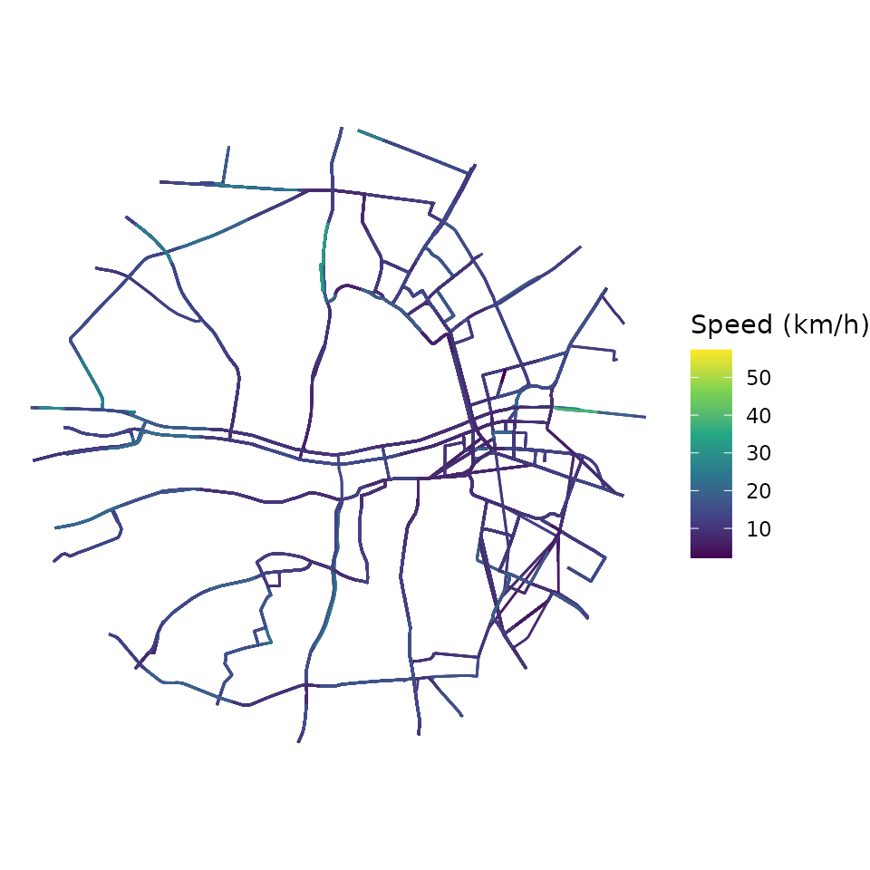
5.2 Fleet data
The next step is to prepare a data.frame with some
characteristics of the public transport fleet. This can be either: - A
simple table with the overall composition of the fleet. In this case,
the gtfs2emis will assume that fleet is homogeneously
distributed across all routes; OR - A detailed table that (1) brings
info on the characteristics of each vehicle and, (2) tells the
probability with which each vehicle type is allocated to each transport
route.
In this introductory vignette, we’ll be working with a simple table that tells us the proportion of buses in Dublin according to their vehicle type, Euro standard, technology, and fuel. The table looks like this:
fleet_file <- system.file("extdata/irl_dub_fleet.txt", package = "gtfs2emis")
fleet_df <- read.csv(fleet_file)
head(fleet_df)
#>             veh_type euro fuel   N fleet_composition    tech
#> 1 Ubus Std 15 - 18 t  III    D  10        0.00998004       -
#> 2 Ubus Std 15 - 18 t   IV    D 296        0.29540918     SCR
#> 3 Ubus Std 15 - 18 t    V    D 148        0.14770459     SCR
#> 4 Ubus Std 15 - 18 t   VI    D 548        0.54690619 DPF+SCR
Please note different emission factor models may require different
information and that the fleet data.frame needs to be
organized accordingly. In our current example for the city of Dublin,
the fleet data must include certain columns with the fleet
characteristics that are used in the EMEP-EEA emission factor model:
vehicle type, Euro standard, technology, and fuel. To check which
columns and sets of vehicle characteristics are required by a given
emission factor model, check the fleet
data vignette.
5.3 Emission model
In the final step, we use the emission_model{gtfs2emis}
function to estimate the hot exhaust emissions of our public transport
system. Here, the user needs to pass the results from
transport_model(), some fleet data as described above, and
select which emission factor model and pollutants should be considered.
The emission_model() outputs a list with
several vectors and data.frames with emission
estimates and related information such as vehicle variables
(fuel, age, tech,
euro, fleet_composition), travel variables
(slope, load, gps) or pollution
(EF, emi).
emi_list <- emission_model(tp_model = tp_model,
                           ef_model = "ef_europe_emep",
                           fleet_data = fleet_df,
                           pollutant = c("CO2","PM10"),
                           reference_year = 2020
                           )

names(emi_list)
#>  [1] "pollutant"         "veh_type"          "euro"
#>  [4] "fuel"              "tech"              "process"
#>  [7] "slope"             "load"              "speed"
#> [10] "EF"                "emi"               "tp_model"
#> [13] "fleet_composition"
6 Analyzing emission estimates
Sometimes, working with data stored in a long list can be tricky. For
convenience, gtfs2emis package has a few functions to help
users analyze the results of emission estimates. For example, you can
use the emis_to_dt() function to convert the output of
emission_model() from a list to a
data.table format:
emi_dt <- emis_to_dt(emi_list = emi_list,
                     veh_vars = c("veh_type", "euro", "fuel"),
                     pol_vars = "pollutant"
                     )

head(emi_dt)
#>              veh_type   euro   fuel pollutant          emi     process
#>                <char> <char> <char>    <char>      <units>      <char>
#> 1: Ubus Std 15 - 18 t    III      D       CO2 4.465969 [g] hot_exhaust
#> 2: Ubus Std 15 - 18 t    III      D       CO2 4.350602 [g] hot_exhaust
#> 3: Ubus Std 15 - 18 t    III      D       CO2 2.349907 [g] hot_exhaust
#> 4: Ubus Std 15 - 18 t    III      D       CO2 8.523031 [g] hot_exhaust
#> 5: Ubus Std 15 - 18 t    III      D       CO2 7.769610 [g] hot_exhaust
#> 6: Ubus Std 15 - 18 t    III      D       CO2 6.659245 [g] hot_exhaust
Alternatively, the emis_summary() function helps users
summarize emission estimates, aggregating emissions by pollutant, time
of the day, vehicle or road segment (spatial).
6.1 Total emissions by pollutant
emi_by_pol <- emis_summary(emi_list = emi_list,
                                 by = "pollutant")
emi_by_pol
#>    pollutant     process              emi
#>       <char>      <char>          <units>
#> 1:       CO2 hot_exhaust 2.685654e+06 [g]
#> 2:      PM10 hot_exhaust 8.732673e+01 [g]
6.2 Total emissions by vehicle type
The emis_summary() function help users summarize
emission estimates by either veh_type,
pollutant, or time. Using this function, users
can easily:
emi_by_veh <- emis_summary(emi_list = emi_list,
                          by = "vehicle")
head(emi_by_veh)
#>              veh_type pollutant     process              emi
#>                <char>    <char>      <char>          <units>
#> 1: Ubus Std 15 - 18 t       CO2 hot_exhaust 2.685654e+06 [g]
#> 2: Ubus Std 15 - 18 t      PM10 hot_exhaust 8.732673e+01 [g]
It is also possible to summarize emission estimates by other vehicle characteristics AND pollutants.
emi_by_veh <- emis_summary(emi_list = emi_list,
                          by = "vehicle",
                          veh_vars = c("veh_type","euro"))
head(emi_by_veh)
#>              veh_type   euro pollutant     process              emi
#>                <char> <char>    <char>      <char>          <units>
#> 1: Ubus Std 15 - 18 t    III       CO2 hot_exhaust 3.124742e+04 [g]
#> 2: Ubus Std 15 - 18 t     IV       CO2 hot_exhaust 8.889753e+05 [g]
#> 3: Ubus Std 15 - 18 t      V       CO2 hot_exhaust 3.637575e+05 [g]
#> 4: Ubus Std 15 - 18 t     VI       CO2 hot_exhaust 1.401674e+06 [g]
#> 5: Ubus Std 15 - 18 t    III      PM10 hot_exhaust 6.369830e+00 [g]
#> 6: Ubus Std 15 - 18 t     IV      PM10 hot_exhaust 4.237565e+01 [g]

# plot
ggplot(data = emi_by_veh) +
  geom_col(aes(x = euro, y = as.numeric(emi/1000), fill = pollutant),
           color=NA, show.legend = FALSE) +
  labs(y="Total emissions (Kg)", x="Euro standard") +
  facet_wrap(~pollutant, scales = "free", nrow = 2) +
  theme_minimal()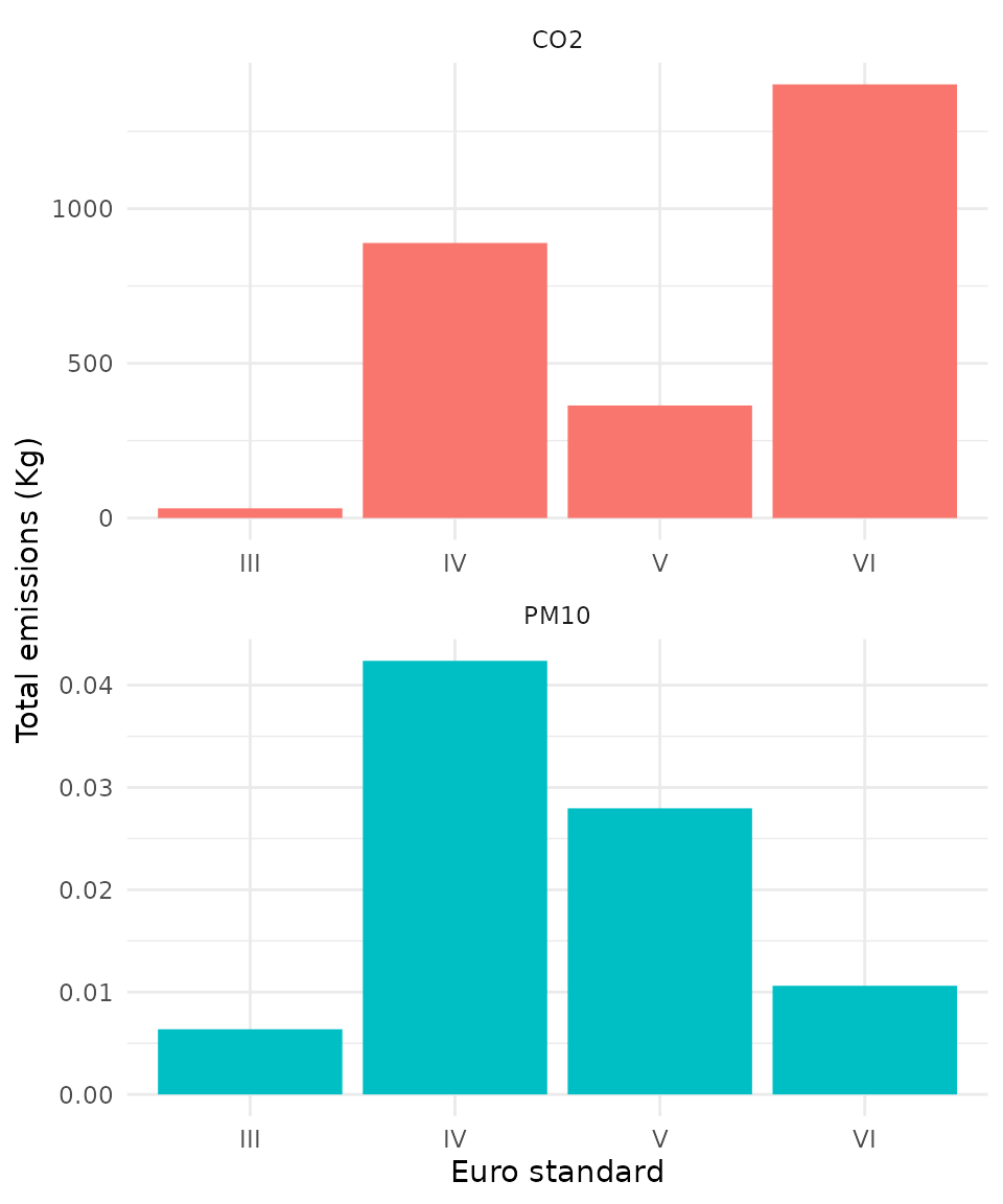
6.3 Total emissions by time of the day
emi_by_time <- emis_summary(emi_list = emi_list,
                                by = "time")
head(emi_by_time)
#>    timestamp_hour pollutant     process          emi
#>             <int>    <char>      <char>      <units>
#> 1:             13       CO2 hot_exhaust 197791.4 [g]
#> 2:             14       CO2 hot_exhaust 235187.9 [g]
#> 3:             15       CO2 hot_exhaust 219913.4 [g]
#> 4:             16       CO2 hot_exhaust 225923.6 [g]
#> 5:             17       CO2 hot_exhaust 318723.4 [g]
#> 6:             18       CO2 hot_exhaust 209437.0 [g]

# plot
ggplot(data = emi_by_time) +
  geom_col(aes(x = factor(timestamp_hour), y = as.numeric(emi/1000), fill = pollutant),
           color=NA, show.legend = FALSE) +
  labs(y="Total emissions (Kg)", x="Hour of the day") +
  facet_wrap(~pollutant, scales = "free", nrow = 2) +
  theme_minimal()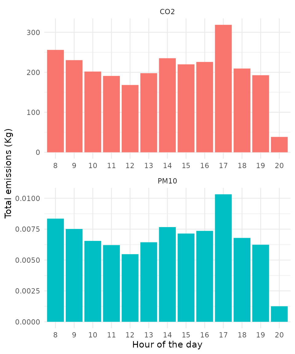
6.4 Spatial distribution of emissions
Finally, users can analyze how public transport emissions are
spatially distributed. To do this, the emis_grid() function
helps aggregate emission estimates over any custom spatial vector data
(sf POLYGON).
Let’s create a regular hexagonal grid for this example.
# create spatial grid
mygrid <- sf::st_make_grid(
  x = sf::st_make_valid(emi_list$tp_model)
  , cellsize = 0.25 / 200
  , crs= 4326
  , what = "polygons"
  , square = FALSE)

 ggplot() +
   geom_sf(data=mygrid) +
   theme_void()
mygrid_emi <- emis_grid(emi_list, mygrid,time_resolution = "day"
                        ,quiet = FALSE)

ggplot() +
  geom_sf(data = mygrid_emi, aes(fill= as.numeric(CO2_Euro_III)), color=NA) +
  geom_sf(data = emi_list$tp_model$geometry,color = "black")+
scale_fill_continuous(type = "viridis")+
  labs(fill = "CO2 (g)")+
  theme_void()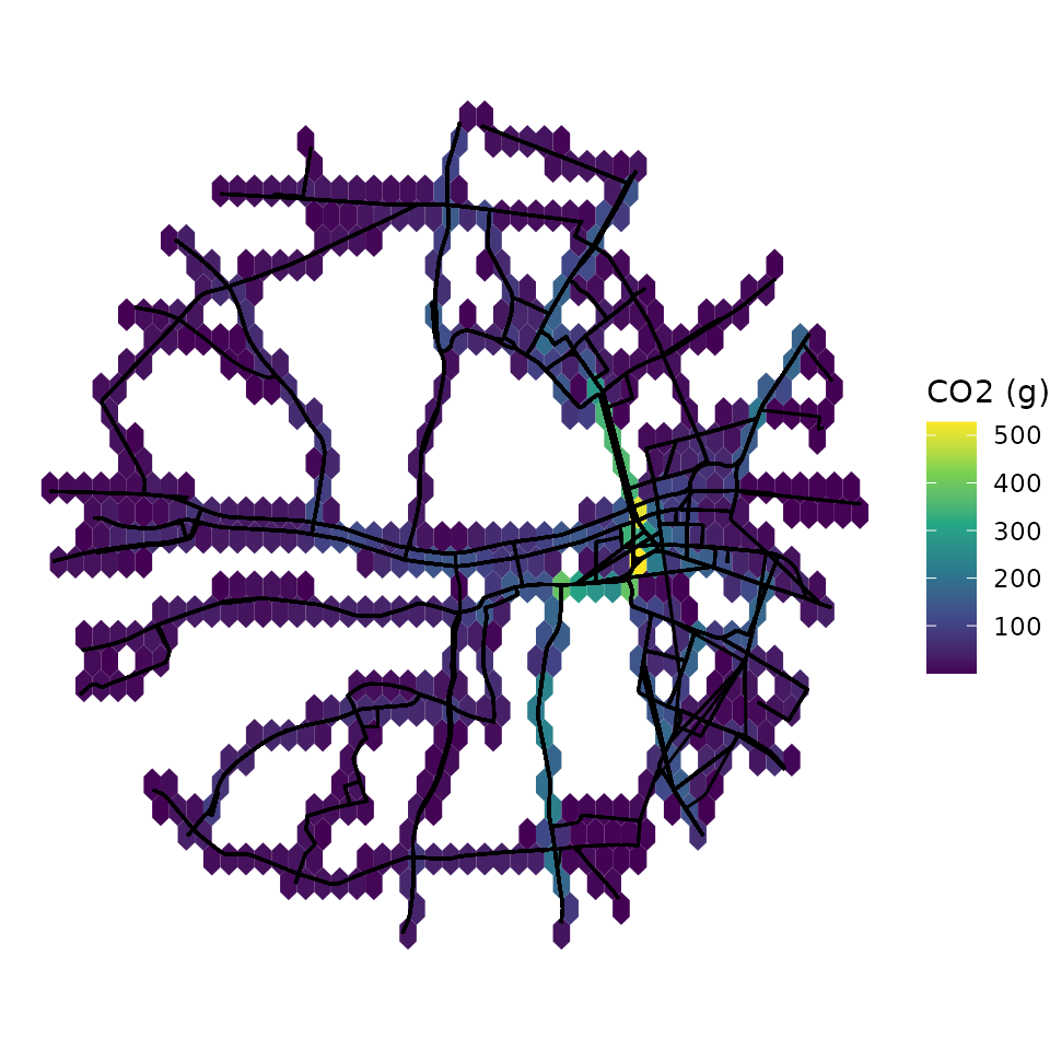
Learn more
Check out our extra guides:
- Defining Fleet data
- Exploring Emission Factors
- Exploring Non-Exhaust Emission Factors ## Report a bug
If you have any suggestions or want to report an error, please visit the package GitHub page.