The General Transit Feed Specification (GTFS) data format defines a common scheme for describing transit systems, and is widely used by transit agencies around the world and consumed by many software applications. The gtfstools package makes handling GTFS data in R very easy and fast, offering many utility functions to read, manipulate, analyze and write transit feeds in such format.
GTFS feeds
GTFS feeds exist in two main different forms: the GTFS
static and the GTFS realtime. This package allows you
to manipulate GTFS static feeds, the most common variation.
These feeds are the collection of many csv-like files (with
a .txt extension) contained in a single .zip
file. A GTFS .zip file is composed by at least five
required files, but may also contain a few other conditionally required
and optional files:
- Required:
agency.txt,stops.txt,routes.txt,trips.txt,stop_times.txt - Conditionally required:
calendar.txt,calendar_dates.txt,feed_info.txt - Optional:
fare_attributes.txt,fare_rules.txt,shapes.txt,frequencies.txt,transfers.txt,pathways.txt,levels.txt,translations.txt,attributions.txt
Please check the official GTFS reference for more details on the specification.
Basic usage
Before using gtfstools please make sure that you have it installed in your computer. You can download either the most stable version from CRAN…
install.packages("gtfstools")…or the development version from GitHub.
install.packages("gtfstools", repos = "https://dhersz.r-universe.dev")

# or
# install.packages("remotes")
remotes::install_github("ipeaGIT/gtfstools")
Then attach it to the current R session:
A few sample files are included in the package:
data_path <- system.file("extdata", package = "gtfstools")
list.files(data_path)
#> [1] "ber_gtfs.zip" "ggl_gtfs.zip" "poa_gtfs.zip" "spo_gtfs.zip"-
ggl_gtfs.ziphas been manually built from the example GTFS feed provided by Google. The files samples are licensed under Creative Commons Attribution 4.0 License. -
spo_gtfs.zipis a subset of the São Paulo’s SPTrans feed, available here. -
ber_gtfs.zipis a subset of Berlin’s GTFS, available here. -
poa_gtfs.zipis a subset of Porto Alegre’s EPTC feed, available here.
Throughout this demonstration we will be using São Paulo’s and Google’s feeds.
Read feeds
gtfstools reads feeds as a list of
data.tables, a high-performance version of base
R’s data.frames. Thus, reading, writing
and manipulating GTFS objects created by gtfstools is
very easy and fast even if some of your tables contain a few million
rows.
To read a feed use the read_gtfs() function. By default
the function reads all .txt files contained in the main
.zip file. It may be useful, however, to read only a couple
of specific files, specially if you’re dealing with some big data sets.
To do so, specify which file you want to read in the files
argument (without the .txt extension):
spo_path <- file.path(data_path, "spo_gtfs.zip")

# default behaviour
spo_gtfs <- read_gtfs(spo_path)
names(spo_gtfs)
#> [1] "agency"      "calendar"    "frequencies" "routes"      "shapes"
#> [6] "stop_times"  "stops"       "trips"

# only reads the 'shapes.txt' and 'trips.txt' files
spo_shapes <- read_gtfs(spo_path, files = c("shapes", "trips"))
names(spo_shapes)
#> [1] "shapes" "trips"
Please note that date fields are read as columns of class
Date, instead of being kept as integers (as specified in
the official
reference), allowing for easier data manipulation. These columns are
converted back to integers when writing the GTFS
objects to a .zip file, so GTFS files generated by the
package always conform to the specification.
Analyse feeds
gtfstools also includes a few functions to prevent you from getting stuck with repetitive tasks:
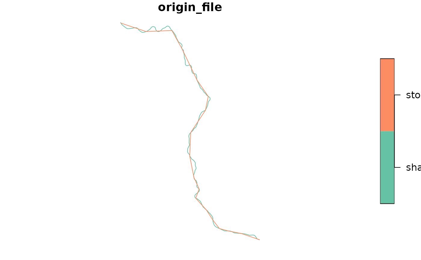
get_trip_geometry() returns the geometry of each trip in
a GTFS object as an sf object (please check {sf} webpage for
more details). GTFS data allows you to generate geometries using two
different methods: either converting the shapes described in the
shapes.txt file to an sf, or linking the
subsequent stops of each trip as described in the
stop_times.txt along a straight line. While the former
tends to yield more reliable and higher resolution geometries, it may be
useful to compare the results of both methods to check if the trips
described in stop_times actually resemble their actual
shape:
trip_geom <- get_trip_geometry(spo_gtfs, file = "shapes")
plot(trip_geom$geometry)
single_trip <- spo_gtfs$trips$trip_id[1]
single_trip
#> [1] "CPTM L07-0"

# 'file' argument defaults to c("shapes", "stop_times")
both_geom <- get_trip_geometry(spo_gtfs, trip_id = single_trip)
plot(both_geom["origin_file"])
get_trip_duration() returns the duration of each trip in
a GTFS object, as specified in the stop_times file, in the
temporal unit of your desire (either seconds, minutes, hours or
days):
trip_durtn <- get_trip_duration(spo_gtfs, unit = "s")
head(trip_durtn)
#> Key: <trip_id>
#>      trip_id duration
#>       <char>    <int>
#> 1: 2002-10-0     2880
#> 2: 2105-10-0     6480
#> 3: 2105-10-1     6660
#> 4: 2161-10-0     5640
#> 5: 2161-10-1     5580
#> 6: 4491-10-0     4140

# 'unit' argument defaults to "min"
single_durtn <- get_trip_duration(spo_gtfs, trip_id = single_trip)
single_durtn
#> Key: <trip_id>
#>       trip_id duration
#>        <char>    <num>
#> 1: CPTM L07-0      136
get_trip_segment_duration() is a similar function, that
even takes the same arguments, but returns the duration of each trip
segment (i.e. the time interval between two consecutive
stops).
trip_seg_durtn <- get_trip_segment_duration(spo_gtfs, unit = "s")
head(trip_seg_durtn)
#>       trip_id segment duration
#>        <char>   <int>    <int>
#> 1: CPTM L07-0       1      480
#> 2: CPTM L07-0       2      480
#> 3: CPTM L07-0       3      480
#> 4: CPTM L07-0       4      480
#> 5: CPTM L07-0       5      480
#> 6: CPTM L07-0       6      480

single_seg_durtn <- get_trip_segment_duration(spo_gtfs, trip_id = single_trip)
head(single_seg_durtn)
#>       trip_id segment duration
#>        <char>   <int>    <num>
#> 1: CPTM L07-0       1        8
#> 2: CPTM L07-0       2        8
#> 3: CPTM L07-0       3        8
#> 4: CPTM L07-0       4        8
#> 5: CPTM L07-0       5        8
#> 6: CPTM L07-0       6        8
The quick example above shows how this function may help you
diagnosing some problems in your GTFS data: apparently every single trip
in spo_gtfs is composed by several equally long segments,
which looks unreasonable.
Finally, get_trip_speed() is a helper around
get_trip_geometry() and get_trip_duration()
that returns the average speed of each trip in a GTFS object:
trip_speed <- get_trip_speed(spo_gtfs, unit = "m/s")
head(trip_speed)
#>      trip_id origin_file    speed
#>       <char>      <char>    <num>
#> 1: 2002-10-0      shapes 2.486809
#> 2: 2105-10-0      shapes 2.848157
#> 3: 2105-10-1      shapes 2.720915
#> 4: 2161-10-0      shapes 3.106259
#> 5: 2161-10-1      shapes 3.273461
#> 6: 4491-10-0      shapes 3.667656

# 'unit' argument defaults to "km/h"
single_trip_speed <- get_trip_speed(spo_gtfs, trip_id = single_trip)
single_trip_speed
#>       trip_id origin_file    speed
#>        <char>      <char>    <num>
#> 1: CPTM L07-0      shapes 26.78777
Manipulate feeds
Each table inside a GTFS object can be easily manipulated using the
usual data.table syntax. data.table provides
many useful features, such as updating columns by reference, fast binary
search, efficient data aggregation, and many others, allowing you to
deal with large data sets very efficiently. Please check its official
website for more details on syntax and usage.
Just remember that, since every GTFS object is a
list of data.tables, you must refer
to each table using the $ operator. For example, this is
how you’d remove the headway_secs column from the
frequencies file and add it again afterwards:
old_headway_secs <- spo_gtfs$frequencies$headway_secs

spo_gtfs$frequencies[, headway_secs := NULL]
head(spo_gtfs$frequencies)
#>       trip_id start_time end_time
#>        <char>     <char>   <char>
#> 1: CPTM L07-0   04:00:00 04:59:00
#> 2: CPTM L07-0   05:00:00 05:59:00
#> 3: CPTM L07-0   06:00:00 06:59:00
#> 4: CPTM L07-0   07:00:00 07:59:00
#> 5: CPTM L07-0   08:00:00 08:59:00
#> 6: CPTM L07-0   09:00:00 09:59:00

spo_gtfs$frequencies[, headway_secs := old_headway_secs]
head(spo_gtfs$frequencies)
#>       trip_id start_time end_time headway_secs
#>        <char>     <char>   <char>        <int>
#> 1: CPTM L07-0   04:00:00 04:59:00          720
#> 2: CPTM L07-0   05:00:00 05:59:00          360
#> 3: CPTM L07-0   06:00:00 06:59:00          360
#> 4: CPTM L07-0   07:00:00 07:59:00          360
#> 5: CPTM L07-0   08:00:00 08:59:00          360
#> 6: CPTM L07-0   09:00:00 09:59:00          480
gtfstools also provides some functions that help you
getting over some common tasks. merge_gtfs() takes many
GTFS objects and combines them row-wise. By default the function binds
every table inside the objects, but you can specify which tables you
want to merge with the files argument:
ggl_path <- file.path(data_path, "ggl_gtfs.zip")
ggl_gtfs <- read_gtfs(ggl_path)

names(spo_gtfs)
#> [1] "agency"      "calendar"    "frequencies" "routes"      "shapes"
#> [6] "stop_times"  "stops"       "trips"
names(ggl_gtfs)
#>  [1] "calendar_dates"  "fare_attributes" "fare_rules"      "feed_info"
#>  [5] "frequencies"     "levels"          "pathways"        "routes"
#>  [9] "shapes"          "stop_times"      "stops"           "transfers"
#> [13] "translations"    "trips"           "agency"          "attributions"
#> [17] "calendar"

merged_gtfs <- merge_gtfs(spo_gtfs, ggl_gtfs)
names(merged_gtfs)
#>  [1] "agency"          "calendar"        "frequencies"     "routes"
#>  [5] "shapes"          "stop_times"      "stops"           "trips"
#>  [9] "calendar_dates"  "fare_attributes" "fare_rules"      "feed_info"
#> [13] "levels"          "pathways"        "transfers"       "translations"
#> [17] "attributions"

# only merges the 'shapes' and 'trips' tables
merged_files <- merge_gtfs(spo_gtfs, ggl_gtfs, files = c("shapes", "trips"))
names(merged_files)
#> [1] "shapes" "trips"
set_trip_speed() sets the average speed of specified
trips by adjusting the arrival_time and
departure_time columns in the stop_times
table. Average speed is calculated as the difference between the arrival
time at the last stop minus the departure time at the first top, divided
by the trip’s length. Please note that arrival and departure times at
intermediate stops are set as "". Some transport routing
software, such as OpenTripPlanner and R5, support specifying stop
times like so, in which case they interpolate arrival/departure times at
intermediate stops based on the trip’s average speed and the euclidean
distance between stops.
selected_trips <- c("2002-10-0", "CPTM L07-0")

get_trip_speed(spo_gtfs, selected_trips, unit = "km/h")
#>       trip_id origin_file     speed
#>        <char>      <char>     <num>
#> 1:  2002-10-0      shapes  8.952511
#> 2: CPTM L07-0      shapes 26.787768

# 'speed' is recycled to all trips if only a single value is given
new_speed_gtfs <- set_trip_speed(spo_gtfs, selected_trips, 50)
get_trip_speed(new_speed_gtfs, selected_trips)
#>       trip_id origin_file    speed
#>        <char>      <char>    <num>
#> 1:  2002-10-0      shapes 50.06453
#> 2: CPTM L07-0      shapes 50.00874

# but you can also specify different speeds for each trip
new_speed_gtfs <- set_trip_speed(spo_gtfs, selected_trips, c(30, 40))
get_trip_speed(new_speed_gtfs, selected_trips)
#>       trip_id origin_file    speed
#>        <char>      <char>    <num>
#> 1:  2002-10-0      shapes 30.01541
#> 2: CPTM L07-0      shapes 40.00516
Write feeds
Finally, write_gtfs() allows you to save your GTFS
objects to disk. It defaults to writing every single table inside the
object as a .txt file, but you can conditionally exclude
files if you so wish:
temp_dir <- file.path(tempdir(), "gttools_vig")
dir.create(temp_dir)
list.files(temp_dir)
#> character(0)

filename <- file.path(temp_dir, "spo_gtfs.zip")

write_gtfs(spo_gtfs, filename)
list.files(temp_dir)
#> [1] "spo_gtfs.zip"
zip::zip_list(filename)$filename
#> [1] "agency.txt"      "calendar.txt"    "frequencies.txt" "routes.txt"
#> [5] "shapes.txt"      "stop_times.txt"  "stops.txt"       "trips.txt"

write_gtfs(spo_gtfs, filename, files = c("stop_times", "trips", "calendar"))
zip::zip_list(filename)$filename
#> [1] "stop_times.txt" "trips.txt"      "calendar.txt"
write_gtfs() also converts Date columns
back to integer, producing GTFS files that conform to the official
specification.
