The geobr package provides quick and easy access to official spatial data sets of Brazil. The package offers a wide range of spatial data sets available at various geographic scales and for various years with harmonized attributes, projection and fixed topology. All geobr functions follow a simple and consistent syntax that allows users to seamlessly download data and work with it either in memory using sf or out of memory using DuckDB and Arrow. This vignette presents a quick intro to geobr.
Installation
You can install geobr from CRAN or the development version to use the latest features.
# From CRAN
install.packages("geobr")

# Development version
utils::remove.packages('geobr')
devtools::install_github("ipeaGIT/geobr", subdir = "r-package")
Now let’s load the libraries we’ll use in this vignette.
General usage
Available data sets
The geobr package currently covers 30 spatial data sets, including a
variety of political-administrative and statistical areas used in
Brazil. You can view what data sets are available using the
list_geobr() function.
# Available data sets
datasets <- list_geobr(wide = TRUE)

head(datasets)
#>                  Function                        geography           source
#> 1             read_amazon            Brazil's Legal Amazon              MMA
#> 2             read_biomes                           Biomes             IBGE
#> 3       read_census_tract  Census tract (setor censitário)             IBGE
#> 4 read_conservation_units Environmental Conservation Units              MMA
#> 5            read_country                          Country             IBGE
#> 6 read_disaster_risk_area              Disaster risk areas CEMADEN and IBGE
#>                                                                                                                                                               year
#> 1                                                                                                                                     2019, 2020, 2021, 2022, 2024
#> 2                                                                                                                                                 2006, 2019, 2025
#> 3                                                                                                                                                 2000, 2010, 2022
#> 4                                                                                                                                                   202402, 202503
#> 5 1872, 1900, 1911, 1920, 1933, 1940, 1950, 1960, 1970, 1980, 1991, 2000, 2001, 2010, 2013, 2014, 2015, 2016, 2017, 2018, 2019, 2020, 2021, 2022, 2023, 2024, 2025
#> 6                                                                                                                                                             2010
Basic syntax
The syntax of all geobr functions operate on the same simple logic, so the code to download the data becomes intuitive for the user. Here are a few examples.
Download an specific geographic area at a given year:
# State of Sergipe
state <- read_state(
  year = 2022,
  code_state = "SE",
  showProgress = FALSE
  )

# Municipality of Sao Paulo
muni <- read_municipality(
  year = 2022,
  code_muni = 3550308,
  showProgress = FALSE
  )

ggplot() +
  geom_sf(data = muni, color=NA, fill = '#1ba185') +
  theme_void()
Download all geographic areas within a state at a given year:
# All municipalities in the state of Minas Gerais
muni <- read_municipality(
  year = 2022,
  code_muni = "MG",
  showProgress = FALSE
  )

head(muni)
If the parameter code_ is not passed to the function,
geobr returns the data for the whole country by default.
# read all schools
inter <- read_schools(
  year = 2022,
  showProgress = FALSE
  )

# read all states
states <- read_state(
  year = 2025,
  showProgress = FALSE
  )

head(states)
#> Simple feature collection with 6 features and 6 fields
#> Geometry type: GEOMETRY
#> Dimension:     XY
#> Bounding box:  xmin: -73.98681 ymin: -13.6937 xmax: -46.06151 ymax: 5.26962
#> Geodetic CRS:  SIRGAS 2000
#> # A tibble: 6 × 7
#>   code_state name_state abbrev_state code_region name_region  year
#>        <dbl> <chr>      <chr>              <dbl> <chr>       <dbl>
#> 1         11 Rondônia   RO                     1 Norte        2025
#> 2         12 Acre       AC                     1 Norte        2025
#> 3         13 Amazonas   AM                     1 Norte        2025
#> 4         14 Roraima    RR                     1 Norte        2025
#> 5         15 Pará       PA                     1 Norte        2025
#> 6         16 Amapá      AP                     1 Norte        2025
#> # ℹ 1 more variable: geometry <GEOMETRY [°]>
Important note about data resolution
All functions to download polygon data such as states, municipalities
etc. have a simplified argument. When
simplified = FALSE, geobr returns the original data set
with high resolution at detailed geographic scale (see documentation).
By default, however, simplified = TRUE and geobr returns
data geometries with simplified borders to improve speed of downloading
and plotting the data.
Plot the data
Once you’ve downloaded the data, it is really simple to plot maps
using ggplot2.
# Remove plot axis
no_axis <- theme(axis.title=element_blank(),
                 axis.text=element_blank(),
                 axis.ticks=element_blank())

# Plot all Brazilian states
ggplot() +
  geom_sf(data=states, fill="#2D3E50", color="#FEBF57", size=.15, show.legend = FALSE) +
  labs(subtitle="States", size=8) +
  theme_minimal() +
  no_axis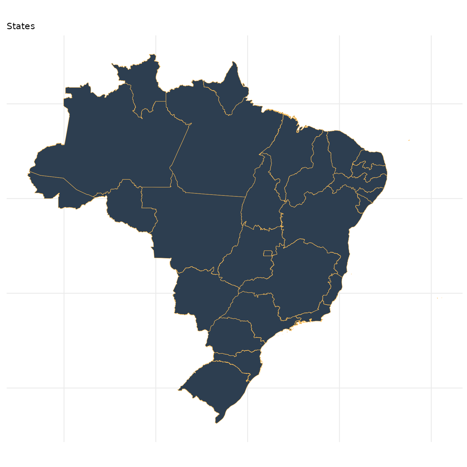
Plot all the municipalities of a particular state, such as Rio de Janeiro:
# Download all municipalities of Rio
all_muni <- read_municipality(
  year= 2022,
  code_muni = "RJ",
  showProgress = FALSE
  )

# plot
ggplot() +
  geom_sf(data=all_muni, fill="#2D3E50", color="#FEBF57", size=.15, show.legend = FALSE) +
  labs(subtitle="Municipalities of Rio de Janeiro, 2000", size=8) +
  theme_minimal() +
  no_axis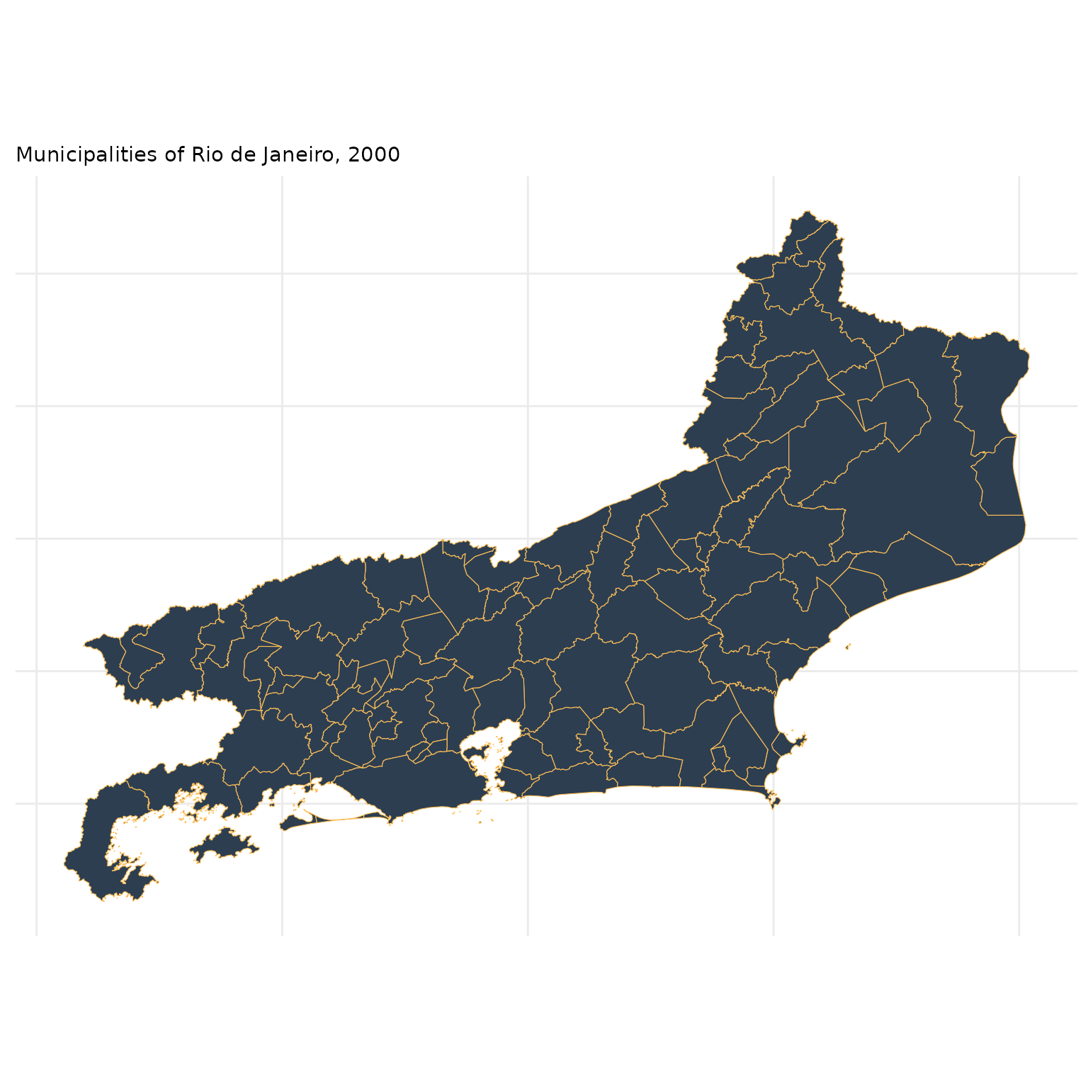
Lazy evaluation with DuckDB and Arrow
By default, all functions in geobr use output = "sf" and
return sf objects loaded into memory. In some cases,
however, it may be preferable to process data out of memory for faster
and more memory-efficient computation, particularly when working with
large spatial data sets.
To support these workflows, users can set
output = "duckdb" to return a lazy
duckspatial_df object. This allows data to be analyzed with
DuckDB using the {duckspatial} package,
enabling efficient out-of-memory spatial operations using a syntax
similar to {sf}.
Alternatively, users can set output = "arrow" to return
an Arrow dataset, which can be integrated with the Arrow ecosystem for
scalable analytical workflows.
# return duckdb duckspatial_df
muni_duck <- geobr::read_municipality(
  year = 2022,
  output = "duckdb"
  )

# return arrow table
muni_arrow <- geobr::read_municipality(
  year = 2022,
  output = "arrow"
  )
Thematic maps
The next step is to combine data from geobr package with other data sets to create thematic maps. In this first example, we will be using data from the (Atlas of Human Development (by Ipea/FJP and UNPD) to create a choropleth map showing the spatial variation of Life Expectancy at birth across Brazilian states.
Merge external data
First, we need a data.frame with estimates of Life
Expectancy. We then need to merge this table to our spatial database.
The two-digit abbreviation of state name is our key column to join these
two data sets.
# Read data.frame with life expectancy data
df <- data.table::fread(
  system.file("extdata/br_states_lifexpect2017.csv", package = "geobr")
  )

# join the databases
states <- dplyr::left_join(
  x = states,
  y = df,
  by = c("name_state" = "uf")
  )
Plot thematic map
ggplot() +
  geom_sf(data=states, aes(fill=ESPVIDA2017), color= NA, size=.15) +
    labs(subtitle="Life Expectancy at birth, Brazilian States, 2014", size=8) +
    scale_fill_distiller(palette = "Blues", name="Life Expectancy", limits = c(65,80)) +
    theme_minimal() +
    no_axis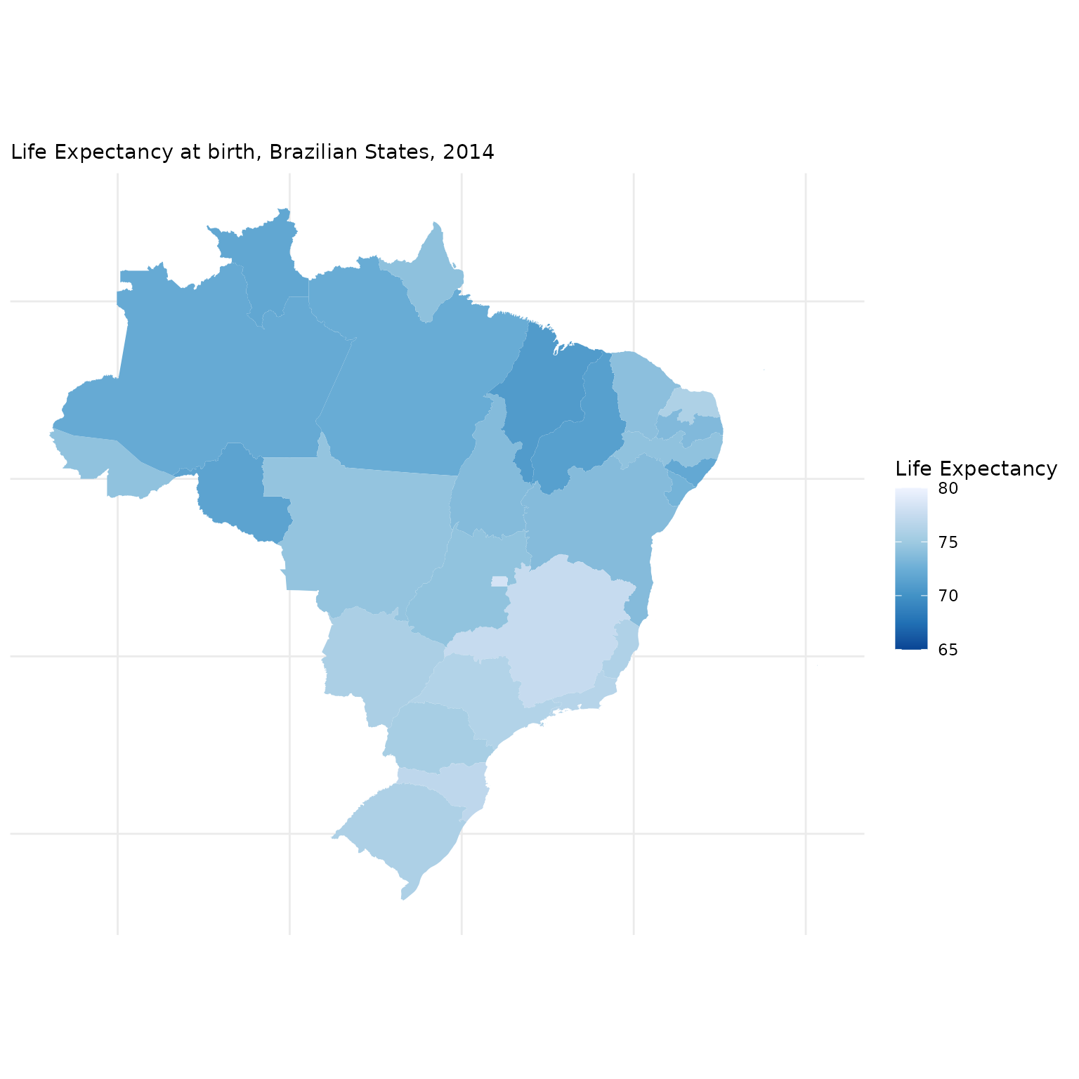
Using geobr together with censobr
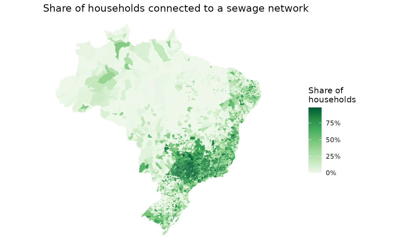
Following the same steps as above, we can use together geobr with our sister package censobr to map the proportion of households connected to a sewage network in Brazilian municipalities
First, we need to download households data from the Brazilian census
using the read_households() function.
library(censobr)
library(arrow)
#>
#> Attaching package: 'arrow'
#> The following object is masked from 'package:utils':
#>
#>     timestamp

hs <- read_households(
  year = 2010,
  showProgress = FALSE
  )
#> ℹ Downloading data and storing it locally for future use.
Now we’re going to (a) group observations by municipality, (b) get the number of households connected to a sewage network, (c) calculate the proportion of households connected, and (d) collect the results.
esg <- hs |>
        collect() |>
        group_by(code_muni) |>                                             # (a)
        summarize(rede = sum(V0010[which(V0207=='1')]),                    # (b)
                  total = sum(V0010)) |>                                   # (b)
        mutate(cobertura = rede / total) |>                                # (c)
        collect()                                                          # (d)

head(esg)
#> # A tibble: 6 × 4
#>   code_muni     rede  total cobertura
#>       <int>    <dbl>  <dbl>     <dbl>
#> 1   1100015     0     7443.   0
#> 2   1100023   182.   27654.   0.00660
#> 3   1100031     0     1979.   0
#> 4   1100049 10019.   24413.   0.410
#> 5   1100056     5.81  5399    0.00108
#> 6   1100064    28.9   6013.   0.00480
Now we only need to download the geometries of Brazilian municipalities from geobr, merge the spatial data with our estimates and map the results.
# download municipality geometries
muni_sf <- geobr::read_municipality(
  year = 2010,
  showProgress = FALSE
  )
#> ℹ Using year/date 2010

# merge data
esg_sf <- left_join(muni_sf, esg, by = 'code_muni')

# plot map
ggplot() +
  geom_sf(data = esg_sf, aes(fill = cobertura), color=NA) +
  labs(title = "Share of households connected to a sewage network") +
  scale_fill_distiller(palette = "Greens", direction = 1,
                       name='Share of\nhouseholds',
                       labels = scales::percent) +
  theme_void()