Spatial aggregation of emission estimates into a grid

Aggregate emissions proportionally in an sf polygon grid, by performing an intersection operation between emissions data in sf linestring format and the input grid cells. User can also aggregate the emissions in the grid by time of the day.

emis_grid(
  emi_list,
  grid,
  time_resolution = "day",
  quiet = TRUE,
  aggregate = FALSE
)

Arguments

emi_list

list. A list containing the data of emissions 'emi' ("data.frame" class) and the transport model 'tp_model' ("sf" "data.frame" classes).

grid

Sf polygon. Grid cell data to allocate emissions.

time_resolution

character. Time resolution in which the emissions is aggregated. Options are 'hour', 'minute', or 'day (Default).

quiet

logical. User can print the total emissions before and after the intersection operation in order to check if the gridded emissions were estimated correctly. Default is 'TRUE'.

aggregate

logical. Aggregate emissions by pollutant. Default is FALSE.

Value

An "sf" "data.frame" object with emissions estimates per grid cell.

See also

Other emission analysis: emis_summary(), emis_to_dt()

Examples

# \donttest{
library(gtfstools)
library(sf)
#> Linking to GEOS 3.8.0, GDAL 3.0.4, PROJ 6.3.1; sf_use_s2() is TRUE

# read GTFS
gtfs_file <- system.file("extdata/bra_cur_gtfs.zip", package = "gtfs2emis")
gtfs <- gtfstools::read_gtfs(gtfs_file) 

# keep a single trip_id to speed up this example
gtfs_small <- gtfstools::filter_by_trip_id(gtfs, trip_id ="4451136")
  
# run transport model
tp_model <- transport_model(gtfs_data = gtfs_small,
                            spatial_resolution = 100,
                            parallel = FALSE)
#> Converting shapes to sf objects
#> Processing the data
#> 
#> Attaching package: ‘data.table’
#> The following object is masked from ‘package:purrr’:
#> 
#>     transpose
#> udunits database from /usr/share/xml/udunits/udunits2.xml

# Fleet data, using Brazilian emission model and fleet
fleet_data_ef_cetesb <- data.frame(veh_type = "BUS_URBAN_D",
                                   model_year = 2010:2019,
                                   fuel = "D",
                                   fleet_composition = rep(0.1,10)
                                   )
# Emission model
emi_list <- emission_model(
                tp_model = tp_model,
                ef_model = "ef_brazil_cetesb",
                fleet_data = fleet_data_ef_cetesb,
                pollutant = c("CO","PM10","CO2","CH4","NOx")
                )
#> Constant emission factor along the route

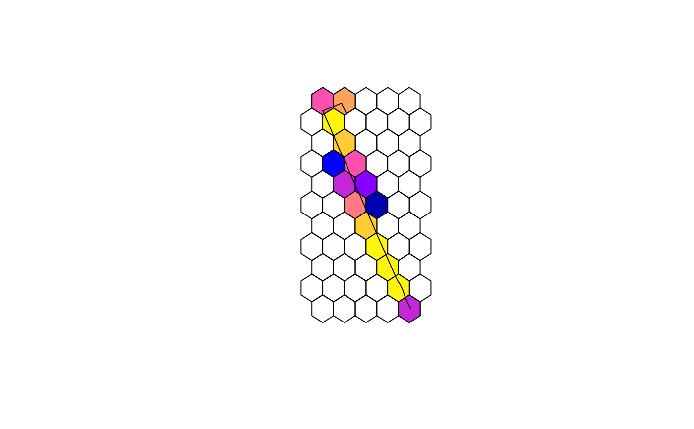
# create spatial grid
grid <- sf::st_make_grid(
  x = sf::st_make_valid(emi_list$tp_model)
  , cellsize = 0.25 / 200
  , crs= 4326
  , what = "polygons"
  , square = FALSE
  )

emi_grid <- emis_grid( emi_list,grid,'day')

plot(grid)
plot(emi_grid["PM10_2010"],add = TRUE)
plot(st_geometry(emi_list$tp_model), add = TRUE,col = "black")

# }