4  GTFS data

The GTFS format is an open and collaborative specification that aims to describe the main components of a public transport network. Originally created in the mid-2000s by a partnership between Google and TriMet, the transport agency of Portland, Oregon, in the United States, the GTFS specification is now used by transport agencies in thousands of cities, spread across all continents of the globe (McHugh 2013). Currently, the specification is divided in two distinct components:

• The GTFS Schedule, or GTFS Static, which contains the planned schedule of public transport trips, information about their fares and spatial information about their itineraries; and
• The GTFS Realtime, which is used to inform, in real-time, vehicle location information, alerts for possible delays, itinerary changes and events that may interfere with the planned schedule.

Throughout this section, we will focus on GTFS Schedule, the most widely used GTFS format in accessibility analyses and by transport agencies¹.

Being an open and collaborative specification, the GTFS format attempts to enable several distinct uses that transport agencies and tool developers might find for it. However, agencies and applications may still depend on information that is not included in the official specification. As a result, different specification extensions have been created, and some of them may eventually be incorporated into the official specification if this is agreed upon by the GTFS community. In this section, we will focus on a subset of information available in the basic GTFS Schedule format, thus not covering its extensions.

4.1 GTFS structure

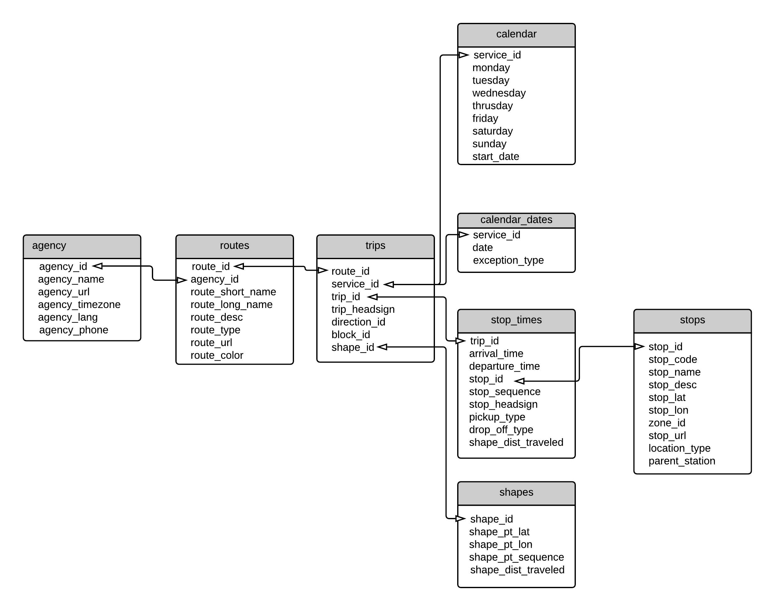
Files in the GTFS Schedule format (from this point onwards referred to as GTFS) are also known as feeds². A feed is nothing more than a compressed .zip file that contains a set of tables, saved in separate .txt files, describing some aspects of the public transport network (stops/stations location, trip frequency, itineraries paths, etc). Just like in a relational database, tables in a feed have key columns that allow one to link information described in one table to the data described in another one. An example of the GTFS scheme is presented in Figure 4.1, which shows some of the the most important tables that make up the specification and highlights the key columns that link the tables together.

Figure 4.1: GTFS format scheme. Source: Pereira, Andrade, and Vieira (2022)

In total, the GTFS format can be made of up to 22 tables³. Some of them, however, are optional, meaning that they don’t need to be present for the feed to be considered valid. The specification classifies the presence of a table into the following categories: required, optional and conditionally required (when the requirement of the table depends on the existence of another particular table, column or value). For simplicity, we will consider only the first two categories in this book and will indicate whether a table is required whenever appropriate. Using our simplified convention, tables are classified as follows:

• Required: agency.txt; stops.txt; routes.txt; trips.txt; stop_times.txt; calendar.txt.
• Optional: calendar_dates.txt: fare_attributes.txt; fare_rules.txt; fare_products.txt; fare_leg_rules.txt; fare_transfer_rules.txt; areas.txt; stop_areas.txt; shapes.txt; frequencies.txt; transfers.txt; pathways.txt; levels.txt; translations.txt; feed_info.txt; attributions.txt.

Throughout this chapter, we will learn about the basic structure of a GTFS file and its tables. We will focus only on the required tables and the optional tables most often used by producers and consumers of these files⁴.

In this demonstration, we use a subset of a feed describing the public transport network of São Paulo, Brazil, produced by São Paulo Transporte (SPTrans)⁵ and downloaded in October 2019. The feed contains the six required tables plus two widely used optional tables, shapes.txt and frequencies.txt, which gives a good overview of the GTFS format.

4.1.1 agency.txt

File used to list the transport operators/agencies running the system described by the feed. Although the term agency, instead of operators, is used, it is up to the feed producer to choose which institutions are listed in the table.

For example, imagine that multiple bus companies operate in a given location, but all schedule and fare planning is carried out by a single institution, either a transport agency or a specific public entity, which is also recognized by public transport users as the system operator. In this case, we should probably list the planning institution in the table.

Now imagine a scenario in which a local public transport agency transfers the operation of a multimodal system to several companies (using concession contracts, for example). Each one of these companies is responsible for planning the schedules and fares of trips/routes they operate, provided that certain pre-established parameters are followed. In this case, we would probably be better off listing the operators in the table, instead of the public transport agency.

Table 4.1 shows the agency.txt file of SPTrans’ feed. We can see that the feed producers decided to list the company itself in the table, instead of the operators of buses and subway routes.

Table 4.1: agency.txt example. Source: SPTrans

agency_id	agency_name	agency_url	agency_timezone	agency_lang
1	SPTRANS	http://www.sptrans.com.br/?versao=011019	America/Sao_Paulo	pt

It is important to note that, although we are presenting agency.txt in table format, the data should be formatted as a .csv file. That is, the values of each cell must be separated by commas, and the contents of each table row must be listed in a different row of the .csv file. The table above, for example, is formatted as follows:

agency_id,agency_name,agency_url,agency_timezone,agency_lang
1,SPTRANS,http://www.sptrans.com.br/?versao=011019,America/Sao_Paulo,pt 

For the sake of communicability and interpretability, the next examples in this chapter are also presented as tables. It is important to keep in mind, however, that these tables are structured as shown above.

4.1.2 stops.txt

File used to describe the stops in a public transport system. The points listed in this file may reference simple stops (such as bus stops), stations, platforms, station entrances and exits, etc. Table 4.2 shows the stops.txt of SPTrans’ feed.

Table 4.2: stops.txt example. Source: SPTrans

stop_id	stop_name	stop_desc	stop_lat	stop_lon
706325	Parada 14 Bis B/C	Viad. Dr. Plínio De Queiroz, 901	-23.55593	-46.65011
810602	R. Sta. Rita, 56	Ref.: R. Bresser / R. João Boemer	-23.53337	-46.61229
910776	Av. Do Estado, 5854	Ref.: Rua Dona Ana Néri	-23.55896	-46.61520
1010092	Parada Caetano Pinto	Av. Rangel Pestana, 1249 Ref.: Rua Caetano Pinto/rua Prof. Batista De Andrade	-23.54615	-46.62218
1010093	Parada Piratininga	Av. Rangel Pestana, 1479 Ref.: Rua Monsenhor Andrade	-23.54509	-46.62006
1010099	R. Xavantes, 612	Ref.: Rua Joli	-23.53545	-46.61368

The columns stop_id and stop_name identify each stop, but fulfill different roles. The purpose of stop_id is to identify relationships between this table and other tables that compose the feed (as we will later see in the stop_times.txt file, for example). Meanwhile, the column stop_name serves as an identifier that should be easily recognized by the passengers, thus usually assuming values of station names, points of interest or addresses (as in the case of SPTrans’ feed).

The stop_desc column, present in SPTrans’ feed, is optional and allows feed producers to add a description of each stop and its surroundings. Finally, stop_lat and stop_lon associate each stop to a point in space with its latitude and longitude geographic coordinates.

Two of the optional columns not present in this stops.txt table are location_type and parent_station. The location_type column is used to indicate the type of location that each point refers to. When not explicitly set, all points are interpreted as public transport stops, but distinct values can be used to distinguish a stop (location_type = 0) from a station (location_type = 1) or a boarding area (location_type = 2), for example. The parent_station column, on the other hand, is used to describe hierarchical relationships between two points. When describing a boarding area, for example, the feed producer must list the stop/platform that this area refers to, and when describing a stop/platform the producer can optionally list the station that it belongs to.

4.1.3 routes.txt

File used to describe the routes that run in a public transport system. Table 4.3 shows the routes.txt of SPTrans’ feed.

Table 4.3: routes.txt example. Source: SPTrans

route_id	agency_id	route_short_name	route_long_name	route_type
CPTM L07	1	CPTM L07	JUNDIAI - LUZ	2
CPTM L08	1	CPTM L08	AMADOR BUENO - JULIO PRESTES	2
CPTM L09	1	CPTM L09	GRAJAU - OSASCO	2
CPTM L10	1	CPTM L10	RIO GRANDE DA SERRA - BRÁS	2
CPTM L11	1	CPTM L11	ESTUDANTES - LUZ	2
CPTM L12	1	CPTM L12	CALMON VIANA - BRAS	2

As in the case of stops.txt, the routes.txt table also includes different columns to distinguish between the identifier of each route (route_id) and their names. In this case, however, there are two distinct name columns: route_short_name and route_long_name. The first refers to the name of the route commonly recognized by passengers, while the second tends to be a more descriptive name. SPTrans, for example, has chosen to highlight the start and endpoints of each route in the latter column. We can also note that the same values are repeated in both route_id and route_short_name, which is neither required nor forbidden - in this case, the feed producer decided that the route names could satisfactorily work as identifiers because they are reasonably short and unique.

The agency_id column works as the key column that links the routes to the data described in agency.txt, and it indicates the agency responsible for operating each route - in this case the agency with id 1 (SPTrans itself). This column is optional in the case of feeds containing a single agency, but required otherwise. Using a feed describing a multimodal system with a subway corridor and several bus lines as an example, a possible configuration of routes.txt could associate the subway routes to the subway operator and the bus routes to the agency/company responsible for planning the bus schedules.

The route_type column is used to describe the transport mode of each route. The above example lists rail lines, whose corresponding numeric value is 2. The corresponding values of other transport modes are listed in the specification.

4.1.4 trips.txt

File used to describe the trips that compose the system. The trip is the basic unit of movement in the GTFS format: each trip is associated with a public transport route (route_id), with a service that operates on certain days of the week (as we will later cover in calendar.txt) and with a spatial trajectory (as we will later cover in shapes.txt). Table 4.4 shows the trips.txt of SPTrans’ feed.

Table 4.4: trips.txt example. Source: SPTrans

trip_id	route_id	service_id	trip_headsign	direction_id	shape_id
CPTM L07-0	CPTM L07	USD	JUNDIAI	0	17846
CPTM L07-1	CPTM L07	USD	LUZ	1	17847
CPTM L08-0	CPTM L08	USD	AMADOR BUENO	0	17848
CPTM L08-1	CPTM L08	USD	JULIO PRESTES	1	17849
CPTM L09-0	CPTM L09	USD	GRAJAU	0	17850
CPTM L09-1	CPTM L09	USD	OSASCO	1	17851

The trip_id column identifies the trips described in the table, just as the route_id references a route described in routes.txt. The service_id column identifies the services that determine the days of the week that each trip runs on (weekdays, weekends, a mix of both, etc), described in detail in calendar.txt. The rightmost column in the example above is shape_id, which identifies the spatial trajectory of each trip, described in detail in the shapes.txt file.

The two remaining columns, trip_headsign and direction_id, are optional and should be used to describe the direction/destination of the trip. The first, trip_headsign, is used to report the text that appears on the vehicle headsign (in the case of buses, for example) or on information panels (such as in subway and rail stations) highlighting the destination of the trip. The direction_id column is often used in conjunction with trip_headsign to distinguish the direction of each trip, where 0 represents one direction and 1 the opposite one. In our example, the first two rows describe trips that refer to the same public transport route (CPTM L07), but in opposite directions: one runs towards Jundiaí, and the other towards Luz.

4.1.5 calendar.txt

File used to describe the different service calendars in a public transport system, listing the set of days of the week in which trips may occur. Each service is also associated to an interval, with a start and an end date, within which the service operates. Table 4.5 shows the calendar.txt of SPTrans’ feed.

Table 4.5: calendar.txt example. Source: SPTrans

service_id	monday	tuesday	wednesday	thursday	friday	saturday	sunday	start_date	end_date
USD	1	1	1	1	1	1	1	20080101	20200501
U__	1	1	1	1	1	0	0	20080101	20200501
US_	1	1	1	1	1	1	0	20080101	20200501
_SD	0	0	0	0	0	1	1	20080101	20200501
__D	0	0	0	0	0	0	1	20080101	20200501
_S_	0	0	0	0	0	1	0	20080101	20200501

The column service_id identifies each service described in the table. As shown earlier, this identifier is also used in the trips.txt, where it associates each trip to a particular service.

The monday, tuesday, wednesday, thursday, friday, saturday and sunday columns are used to list the days of the week in which each service operates. A value of 1 means that the service operates on that day, while a value of 0 means that it does not. In the example above, the USD service operates on every day of the week and the service U__ operates only on business days.

Finally, the columns start_date and end_date delimit the interval within which the services are valid. Dates in GTFS files must always be formatted using the YYYYMMDD format: the first four numbers define the year, the subsequent two define the month and the last two, the day. The value 20220428, for example, represents the 28th of April 2022.

4.1.6 shapes.txt

File used to describe the spatial trajectory of each trip in the system. This file is optional, but feed producers are strongly encouraged to include it in their GTFS files. Table 4.6 shows the shapes.txt of SPTrans’ feed.

Table 4.6: shapes.txt example. Source: SPTrans

shape_id	shape_pt_lat	shape_pt_lon	shape_pt_sequence
17846	-23.53517	-46.63535	1
17846	-23.53513	-46.63548	2
17846	-23.53494	-46.63626	3
17846	-23.53473	-46.63710	4
17846	-23.53466	-46.63735	5
17846	-23.53416	-46.63866	6

The column shape_id identifies each shape and links each trip to its spatial trajectory in the trips.txt table. Unlike all the other identifiers we have seen so far, however, shape_id is repeated in several table rows. This is because each shape is defined by a sequence of spatial points, whose geographic coordinates are described with the shape_pt_lat and shape_pt_lon columns. The shape_pt_sequence column lists the sequence in which the points connect to form the shape. Values listed in this column must increase along the path.

4.1.7 stop_times.txt

File used to describe the timetable of each trip, including the arrival and departure times at each stop. How this table should be formatted depends on whether the feed contains a frequencies.txt table or not, a detail that we will cover later. For now, we will look at the stop_times.txt of SPTrans’ feed, which also includes a frequencies.txt, in Table 4.7.

Table 4.7: stop_times.txt example. Source: SPTrans

trip_id	arrival_time	departure_time	stop_id	stop_sequence
CPTM L07-0	04:00:00	04:00:00	18940	1
CPTM L07-0	04:08:00	04:08:00	18920	2
CPTM L07-0	04:16:00	04:16:00	18919	3
CPTM L07-0	04:24:00	04:24:00	18917	4
CPTM L07-0	04:32:00	04:32:00	18916	5
CPTM L07-0	04:40:00	04:40:00	18965	6

The trip whose timetable is being described is identified by the trip_id column. Similarly to what happens in shapes.txt, the same trip_id appears in several rows. This is because, just like a trip trajectory is composed of a sequence of spatial points, a timetable consists of a sequence of departure/arrival times at various public transport stops.

The next columns, arrival_time, departure_time and stop_id, describe the schedule of each trip, associating an arrival and a departure time to each visited stop. The time columns must be formatted using the HH:MM:SS format, with the first two numbers defining the hour, the subsequent two the minutes and the last two, the seconds. This format also accepts hour values greater than 24: for example, if a trip departs at 11 pm but it only arrives at a given station at 1 am of the next day, the arrival time must be listed as 25:00:00, not 01:00:00. The stop_id column associates the arrival and departure times with a stop described in stops.txt and the stop_sequence column lists the sequence in which the stops connect to form the trip schedule. The values of this last column must always increase along the trip.

It is worth highlighting here the difference between shapes.txt and stop_times.txt. Although both tables present some spatial information of the trips, they do it in different ways. The stop_times.txt table lists the sequence of stops and times that make up a schedule, but says nothing about the trajectory traveled between the stops. shapes.txt, on the other hand, describes the detailed trajectory of a trip, but does not specify where the public transport stops are located. Combined, the information from the two tables allows one to understand both the schedule of each trip and the spatial trajectory between stops.

4.1.8 frequencies.txt

Optional file used to describe the frequency of each trip within different time intervals of a day. Table 4.8 shows the frequency.txt of SPTrans’ feed.

Table 4.8: frequencies.txt example. Source: SPTrans

trip_id	start_time	end_time	headway_secs
CPTM L07-0	04:00:00	04:59:00	720
CPTM L07-0	05:00:00	05:59:00	360
CPTM L07-0	06:00:00	06:59:00	360
CPTM L07-0	07:00:00	07:59:00	360
CPTM L07-0	08:00:00	08:59:00	360
CPTM L07-0	09:00:00	09:59:00	480

The trip whose frequency is being described is identified by the trip_id column. Again, the same identifier may appear in multiple observations. This is because the specification allows the same trip to have different frequencies throughout the day, such as at peak and off-peak hours, for example. Thus, each row refers to the frequency of a given trip within the time interval specified by the start_time and end_time columns.

Within this interval, the trip operates on regular headways specified in headway_secs. The headway is the time between trips that operate the same route. In the case of this table, this time must be specified in seconds. In the example above, we see a headway of 720 between 4 and 5 am, which indicates that the CPTM L07-0 trip departs every 12 minutes within this interval.

Using frequencies.txt and stop_times.txt together

It is important to understand how the presence of a frequencies.txt table changes the specification of stop_times.txt. As we can see in the stop_times.txt example, the CPTM L07-0 trip departs from the first stop at 4 am and arrives at the second at 4:08 am. The arrival and departure times at a given stop, however, cannot be specified more than once for each trip, even though the headway set in frequencies.txt defines that this trip departs every 12 minutes from 4 am to 5 am. If that’s the case, how can we set the schedule of trips departing at 4:12 am, 4:24 am, 4:36 am, etc?

If the frequency of a trip is specified in frequencies.txt, the timetable of this trip defined in stop_times.txt should be understood as a reference that describes the time between stops. In other words, the times defined in the stop_times.txt file should not be interpreted “as is”. For example, the timetable of trip CPTM L07-0 establishes that the journey between the first and second stop takes 8 minutes to complete, which is the same travel time between the second and third stops as well. Thus, a trip departing from the first stop at 4 am arrives at the second at 4:08 am and at the third at 4:16 am. The next trip, which departs from the first stop at 4:12 am, arrives at the second stop at 4:20 am and at the third at 4:28 am.

To describe the same trips in stop_times.txt without making a frequencies.txt table, one could add a suffix that would identify each trip of route CPTM L07 in direction 0 throughout the day. The trip with id CPTM L07-0_1, for example, would be the first trip of the day heading towards direction 0 and would depart from the first stop at 4 am and arrive at the second at 4:08 am. The CPTM L07-0_2 trip, on the other hand, would be the second trip of the day and would depart from the first stop at 04:12 am and arrive at the second at 4:20 am. The rest of the trips would follow the same pattern. Each one of these trips would also need to be added to trips.txt, as well as to any other tables that use trip_id.

Another variable that changes how frequencies.txt affects the timetables in stop_times.txt is the optional column exact_times. When it assumes the value of 0 (or when it is missing from the feed, as in the case of the SPTrans’ GTFS file) it indicates that the trip does not necessarily follow a fixed schedule over the time interval. Instead, operators try to maintain a predetermined headway during the interval. Using the same example of a trip whose headway is 12 minutes between 4 am and 5 am, this would mean that the first departure does not necessarily happen at 4 am, the second at 4:12 am, and so on. The first trip can, for example, leave at 4:02 am. The second, at 4:14 am or 4:13 am, etc. Meanwhile, an exact_times value of 1 must be used to define a schedule that always follows the exact same headway. This is an equivalent and more concise way of defining several similar trips departing at different times in stop_times.txt (as shown in the previous paragraph).

4.2 Finding GTFS data for Brazilian cities

GTFS data from cities all over the world can be downloaded with the {tidytransit} R package or on the Transitland website. In Brazil, several cities use GTFS data to plan and operate their transport systems. In many cases, however, the data is owned by private companies and operators and is not publicly available. As a result, GTFS data in Brazil is seldom openly available, which goes against the public interest and against good practices of data management and governance. Table 4.9 lists some of the few Brazilian cities that make their GTFS feeds openly available to the public⁶.

Table 4.9: Openly available GTFS data in Brazil

City	Source	Info
Belo Horizonte	Belo Horizonte’s Transport and Traffic Company (BHTrans)	Open data: conventional transport network and supplementary network.
Fortaleza	Fortaleza’s Urban Transport Company (Etufor)	Open data.
Fortaleza	Fortaleza’s Subway (Metrofor)	Open data.
Porto Alegre	Porto Alegre’s Transport and Traffic Public Company (EPTC)	Open data.
Rio de Janeiro	Municipal Department of Transport (SMTR)	Open data.
São Paulo	São Paulo’s Metropolitan Urban Transport Company (EMTU)	Download link. Registration required.
São Paulo	SPTrans	Download link. Registration required.

Note: The GTFS data provided by SMTR does not include train and subway data.

McHugh, Bibiana. 2013. “Pioneering Open Data Standards: The GTFS Story.” In Beyond Transparency: Open Data and the Future of Civic Innovation, edited by Brett Goldstein and Lauren Dyson, First, 125–35. San Francisco, CA: Code for America Press.

Pereira, Rafael H. M., Pedro R. Andrade, and João Pedro Bazzo Vieira. 2022. “Exploring the Time Geography of Public Transport Networks with the Gtfs2gps Package.” Journal of Geographical Systems, December. https://doi.org/10.1007/s10109-022-00400-x.

---

1. Please visit https://gtfs.org/realtime/ for more information on GTFS Realtime.

2. In this book, we will use the terms feed, GTFS file and GTFS data as synonyms.

3. According to the official specification as of May 9th 2022.

4. For more information on the tables and columns not covered in this section, please check the official specification.

5. Available at https://www.sptrans.com.br/desenvolvedores/.

6. As of the publication date of this book.