GTFS data is frequently used in various types of analyses that involve a few common elements. The AOP team has developed the {gtfstools} R package, which provides several functions that help tackling repetitive tasks and operations and facilitate feed manipulation and exploration.
In this chapter, we’ll go through some of the most frequently used package features. To do this, we will use a sample of the SPTrans feed presented in the previous chapter, and which is included in the package installation.
5.1 Reading and manipulating GTFS files
Reading GTFS files with {gtfstools} is done with the read_gtfs() function, which receives a string with the file path. The package represents a feed as a list of data.tables, a high-performance version of data.frames. Throughout this chapter, we will refer to this list of tables as a GTFS object. By default, the function reads all .txt tables in the feed:
# loads the packagelibrary(gtfstools)# points to path of the sample gtfs data installed in {gtfstools}path <-system.file("extdata/spo_gtfs.zip", package ="gtfstools")# reads the gtfsgtfs <-read_gtfs(path)# checks the tables inside the gtfs objectnames(gtfs)
We can see that each data.table within the GTFS object is named according to the table it represents, without the .txt extension. This configuration allows us to select and manipulate each table individually. The code below, for example, lists the first 6 rows of the trips table:
Tables within a GTFS object can be easily manipulated using the {dplyr} or {data.table} packages, for example. In this book, we opted to use the {data.table} syntax. This package offers several useful features, primarily for manipulating tables with a large number of records, such as updating columns by reference, very fast row subsets and efficient data aggregation1. For example, we can use the code below to add 100 seconds to all the headways listed in the frequencies table and later reverse this change:
# saves original headwaysoriginal_headway <- gtfs$frequencies$headway_secshead(gtfs$frequencies, 3)
After editing a GTFS object in R, we often want to use the processed GTFS to perform different analyses. In order to do this, we frequently need the GTFS file in .zip format again, and not as a list of tables in an R session. To transform GTFS objects that exist in an R session into GTFS files saved to disk, {gtfstools} includes the write_gtfs() function. To use this function, we only need to pass the object that should be written to disk and the file path where it should be written to:
# points to the path where the GTFS should be written toexport_path <-tempfile("new_gtfs", fileext =".zip")# writes the GTFS to the pathwrite_gtfs(gtfs, path = export_path)# lists files within the feedzip::zip_list(export_path)[, c("filename", "compressed_size", "timestamp")]
GTFS files are often used in public transport routing applications and to inform the timetable of different routes in a given region to potential passengers. Feeds must, therefore, accurately describe the schedule and the operational speed of public transport trips.
To calculate the average speed of the trips described in a feed, {gtfstools} package includes the function get_trip_speed(). By default, the function returns the speed (in km/h) of all trips included in the feed, but one can choose to calculate the speed of selected trips with the trip_id parameter:
# calculates the speeds of all tripsspeeds <-get_trip_speed(gtfs)head(speeds)
To calculate the speed of a trip, we need to know its length and how long it takes to travel from its first to its last stop. Behind the scenes, get_trip_speed() uses two other functions from {gtfstools} toolset: get_trip_length() and get_trip_duration(). The usage of both is very similar to what has been shown before, returning the length/duration of all trips by default or of a few selected trips if desired. Below, we show their default behavior:
# calculates the length of all tripslengths <-get_trip_length(gtfs, file ="shapes")head(lengths)
Just as get_trip_speed() returns speeds in km/h by default, get_trip_length() returns lengths in km and get_trip_duration() returns the duration in minutes. These units can be adjusted with the unit parameter, present in all three functions.
5.3 Combining and filtering feeds
The tasks of processing and manipulating GTFS files are often performed manually, which may increase the chances of leaving minor inconsistencies or errors in the data. A common issue in some GTFS feeds is the presence of duplicate records in the same table. SPTrans’ feed, for example, contains duplicate records both in agency.txt and in calendar.txt:
{gtfstools} includes the remove_duplicates() function to keep only unique entries in all tables of the feed. This function takes a GTFS object as input and returns the same object without duplicates:
We often have to deal with multiple feeds describing the same study area. For example, when the bus and the rail systems of a single city are described in separate GTFS files. In such cases, we may want to merge both files into a single feed to reduce the data processing effort. To help us with that, {gtfstools} includes the merge_gtfs() function. The example below shows the output of merging SPtrans’ feed (without duplicate entries) with EPTC’s feed:
# reads Porto Alegre's GTFSpoa_path <-system.file("extdata/poa_gtfs.zip", package ="gtfstools")poa_gtfs <-read_gtfs(poa_path)poa_gtfs$agency
   agency_id                                 agency_name             agency_url
1:      EPTC Empresa Publica de Transportes e Circulação http://www.eptc.com.br
     agency_timezone agency_lang agency_phone
1: America/Sao_Paulo          pt          156
                                                  agency_fare_url
1: http://www2.portoalegre.rs.gov.br/eptc/default.php?p_secao=155
# combines Porto Alegre's and São Paulo's GTFS objectscombined_gtfs <-merge_gtfs(no_dups_gtfs, poa_gtfs)# check resultscombined_gtfs$agency
   agency_id                                 agency_name
1:         1                                     SPTRANS
2:      EPTC Empresa Publica de Transportes e Circulação
                                 agency_url   agency_timezone agency_lang
1: http://www.sptrans.com.br/?versao=011019 America/Sao_Paulo          pt
2:                   http://www.eptc.com.br America/Sao_Paulo          pt
   agency_phone                                                agency_fare_url
1:
2:          156 http://www2.portoalegre.rs.gov.br/eptc/default.php?p_secao=155
We can see that the tables of both feeds are combined into a single one. This is the case when two (or more) GTFS objects contain the same table (agency, in the example). When a particular table is present in only one of the feeds, the function copies this table to the output. That’s the case of the frequencies table, in our example, which exists only in SPTrans’ feed:
Filtering feeds to keep only a few entries within each table is another operation that frequently comes up when dealing with GTFS data. Feeds are often used to describe large-scale public transport networks, which may result in complex and slow data manipulation, analysis and sharing. Thus, planners and researchers often work with feeds’ subsets. If we want to measure the performance of a transport network during the morning peak, for example, we can filter our GTFS data to keep only the observations related to trips that run within this period.
{gtfstools} includes lots of functions to filter GTFS data. They are:
filter_by_agency_id();
filter_by_route_id();
filter_by_service_id();
filter_by_shape_id();
filter_by_stop_id();
filter_by_trip_id();
filter_by_route_type();
filter_by_weekday();
filter_by_time_of_day(); and
filter_by_sf().
5.3.1 Filtering by identifiers
The seven first functions from the above list work very similarly. They take as input a vector of identifiers and return a GTFS object whose table entries are related to the specified ids. The example below demonstrates this functionality with filter_by_trip_id():
# keeps entries related to the two specified idsfiltered_gtfs <-filter_by_trip_id( gtfs,trip_id =c("CPTM L07-0", "CPTM L07-1"))# checks post-filter object sizeutils::object.size(filtered_gtfs)
We can see from the code snippet above that the function not only filters trips, but all other tables containing a column that relates to trip_id in any way. The shapes of trips CPTM L07-0 and CPTM L07-1, for example, are respectively described by shape_ids 17846 and 17847. Therefore, these are the only shape identifiers kept in the filtered GTFS.
The function also supports the opposite behavior: instead of keeping the entries related to the specified identifiers, we can drop them. To do this, we need to set the keep argument to FALSE:
# removes entries related to two trips from the feedfiltered_gtfs <-filter_by_trip_id( gtfs,trip_id =c("CPTM L07-0", "CPTM L07-1"),keep =FALSE)head(filtered_gtfs$trips[, .(trip_id, trip_headsign, shape_id)])
      trip_id       trip_headsign shape_id
1: CPTM L08-0        AMADOR BUENO    17848
2: CPTM L08-1       JULIO PRESTES    17849
3: CPTM L09-0              GRAJAU    17850
4: CPTM L09-1              OSASCO    17851
5: CPTM L10-0 RIO GRANDE DA SERRA    17852
6: CPTM L10-1                BRÁS    17853
We can see that the specified trips, as well as their shapes, are not present in the filtered GTFS anymore. The same logic, demonstrated here with filter_by_trip_id(), applies to the functions that filter GTFS objects by agency_id, route_id, service_id, shape_id, stop_id and route_type.
5.3.2 Filtering by day of the week and time of the day
Another common operation when dealing with GTFS data is subsetting feeds to keep services that only happen during certain times of the day or days of the week. To do this, the package includes the filter_by_weekday() and filter_by_time_of_day() functions.
filter_by_weekday() takes as input the days of the week whose services that operate on them should be kept (or dropped). The function also includes a combine parameter, which defines how multi-days filters should work. When this argument receives the value "and", only services that operate on every single specified day are kept. When it receives the value "or", services that operate on at least one of the days are kept:
# keeps services that operate on both saturday AND sundayfiltered_gtfs <-filter_by_weekday( no_dups_gtfs,weekday =c("saturday", "sunday"),combine ="and")filtered_gtfs$calendar[, c("service_id", "sunday", "saturday")]
   service_id sunday saturday
1:        USD      1        1
2:        _SD      1        1
# keeps services that operate EITHER on saturday OR on sundayfiltered_gtfs <-filter_by_weekday( no_dups_gtfs,weekday =c("sunday", "saturday"),combine ="or")filtered_gtfs$calendar[, c("service_id", "sunday", "saturday")]
filter_by_time_of_day(), on the other hand, takes the beginning and the end of a time window and keeps (or drops) the entries related to the trips that run within this window. The behavior of this function depends on whether a frequencies table is included in the feed or not: the stop_times timetable of trips listed in frequencies must not be filtered, because, as previously mentioned, it works as a reference that describes the time between consecutive stops, and the departure and arrival times listed there should not be considered rigorously. If a trip is not listed in frequencies, however, its stop_times entries are filtered according to the specified time window. Let’s see how the function works with some examples:
# keeps trips that run within the 5am to 6am windowfiltered_gtfs <-filter_by_time_of_day(gtfs, from ="05:00:00", to ="06:00:00")head(filtered_gtfs$frequencies)
# save the frequencies table and remove it from the original gtfsfrequencies <- gtfs$frequenciesgtfs$frequencies <-NULLfiltered_gtfs <-filter_by_time_of_day(gtfs, from ="05:00:00", to ="06:00:00")head(filtered_gtfs$stop_times[, c("trip_id", "departure_time", "arrival_time")])
Filtering the stop_times table can work in two different ways. One is to keep trips that cross the specified time window intact. The other is to keep only the timetable entries that take place inside this window (default behavior). This behavior is controlled by the full_trips parameter, as shown below (please pay attention to the times and stops present in each example):
# keeps any trips that cross the 5am to 6am window intactfiltered_gtfs <-filter_by_time_of_day( gtfs,from ="05:00:00", to ="06:00:00",full_trips =TRUE)head( filtered_gtfs$stop_times[ ,c("trip_id", "departure_time", "arrival_time", "stop_sequence") ])
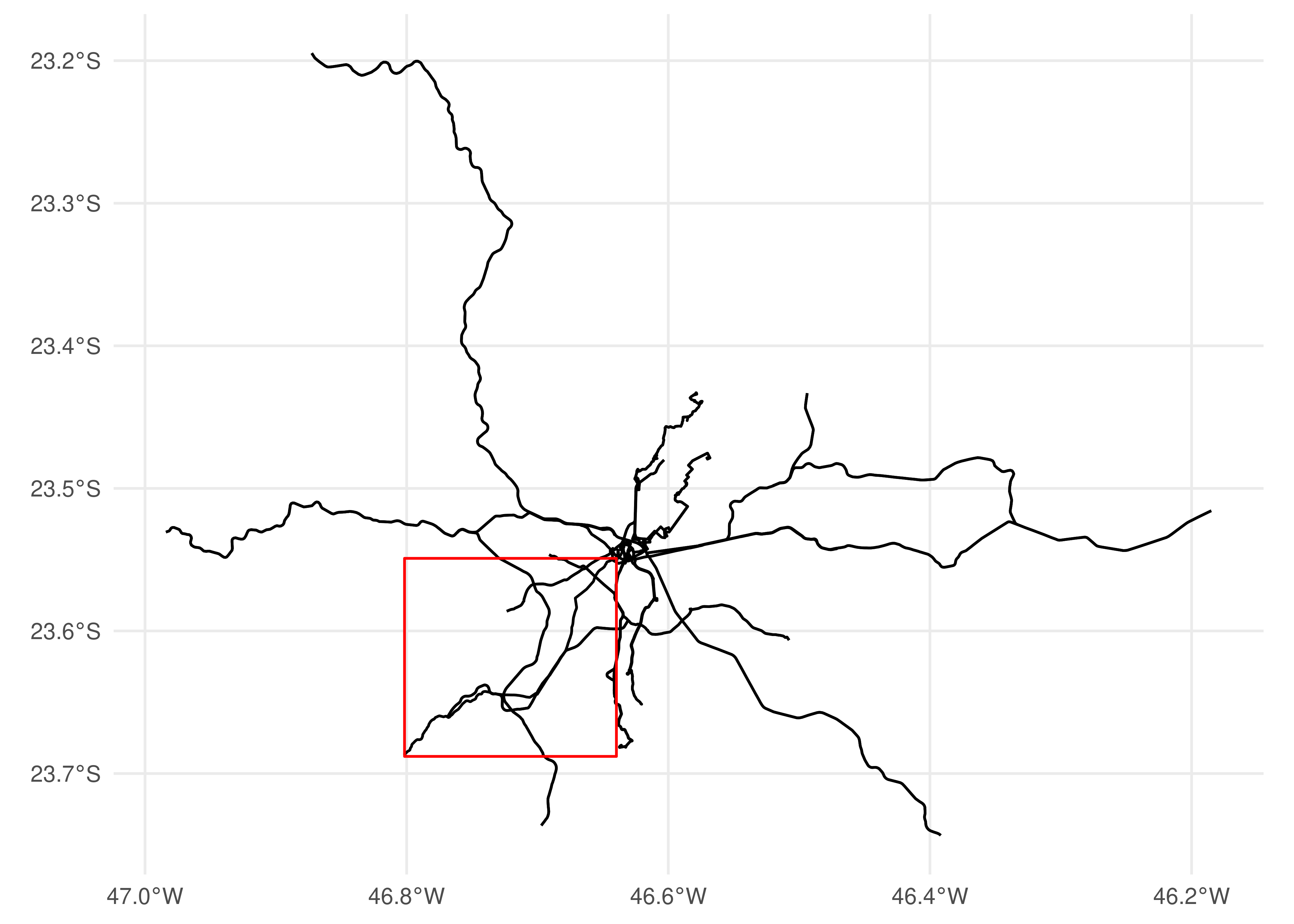
Finally, {gtfstools} also includes a function that allows one to filter a GTFS object using a spatial polygon. filter_by_sf() takes an sf/sfc object (spatial representation created by the {sf} package), or its bounding box, and keeps the entries related to trips selected by their position in relation to that spatial polygon. Although this might seem complicated, this filtering process is fairly easy to grasp once we illustrate it with an example. To demonstrate this function, we are going to filter SPTrans’ feed using the bounding box of shape 68962. With the code snippet below we show the spatial distribution of unfiltered data along with the bounding box in red:
library(ggplot2)# creates a polygon with the bounding box of shape 68962shape_68962 <-convert_shapes_to_sf(gtfs, shape_id ="68962")bbox <- sf::st_bbox(shape_68962)bbox_geometry <- sf::st_as_sfc(bbox)# creates a geometry with all the shapes described in the gtfsall_shapes <-convert_shapes_to_sf(gtfs)ggplot() +geom_sf(data = all_shapes) +geom_sf(data = bbox_geometry, fill =NA, color ="red") +theme_minimal()
Figure 5.1: Shapes spatial distribution overlayed by the bounding box of shape 68962
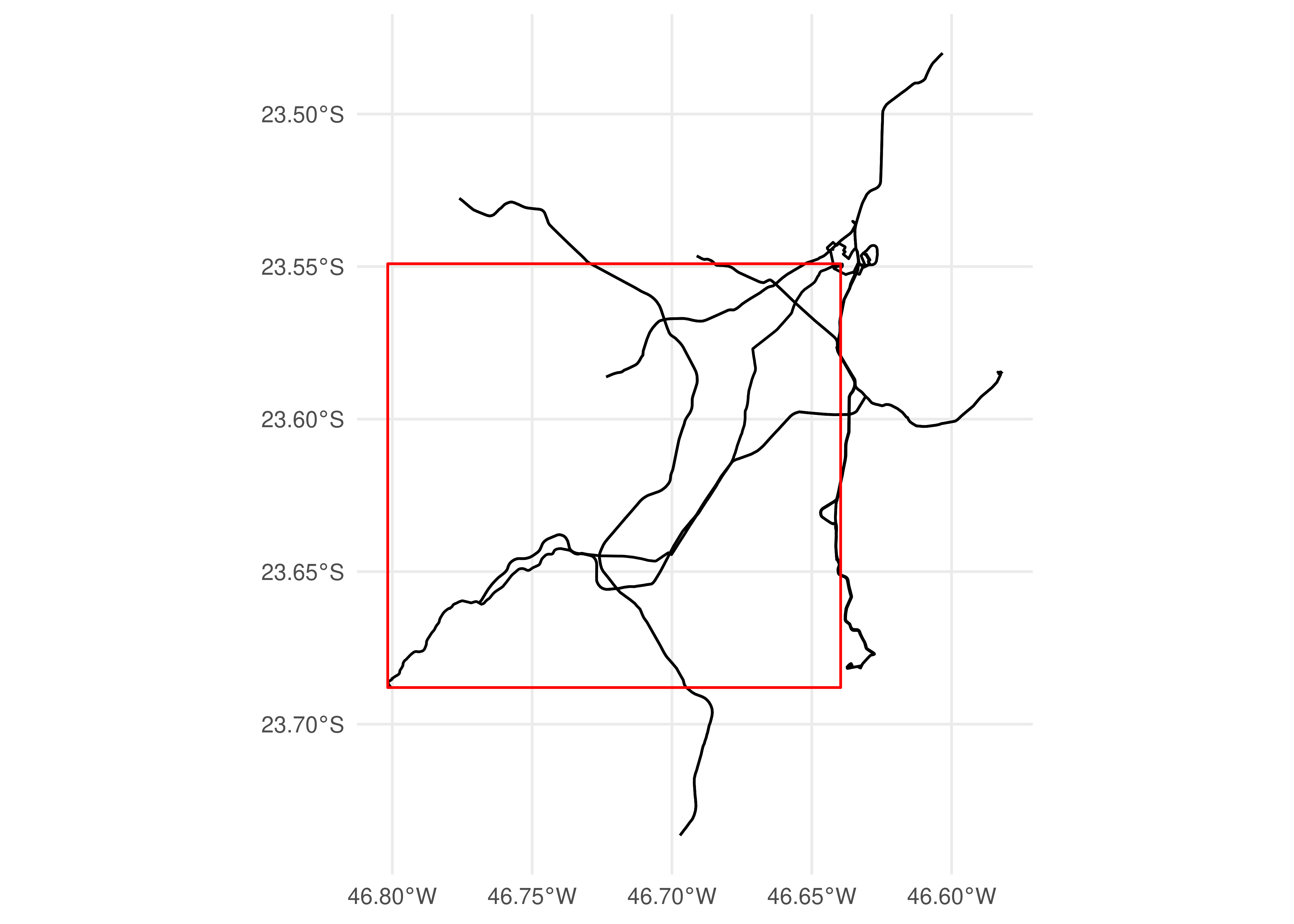
Please note that we have used the convert_shapes_to_sf() function, also included in {gtfstools}, to convert the shapes described in the feed into a sf spatial object. By default, filter_by_sf() keeps all entries related to trips that intersect with the specified polygon:
filtered_gtfs <-filter_by_sf(gtfs, bbox)filtered_shapes <-convert_shapes_to_sf(filtered_gtfs)ggplot() +geom_sf(data = filtered_shapes) +geom_sf(data = bbox_geometry, fill =NA, color ="red") +theme_minimal()
Figure 5.2: Spatial distribution of shapes that intersect with the bounding box of shape 68962
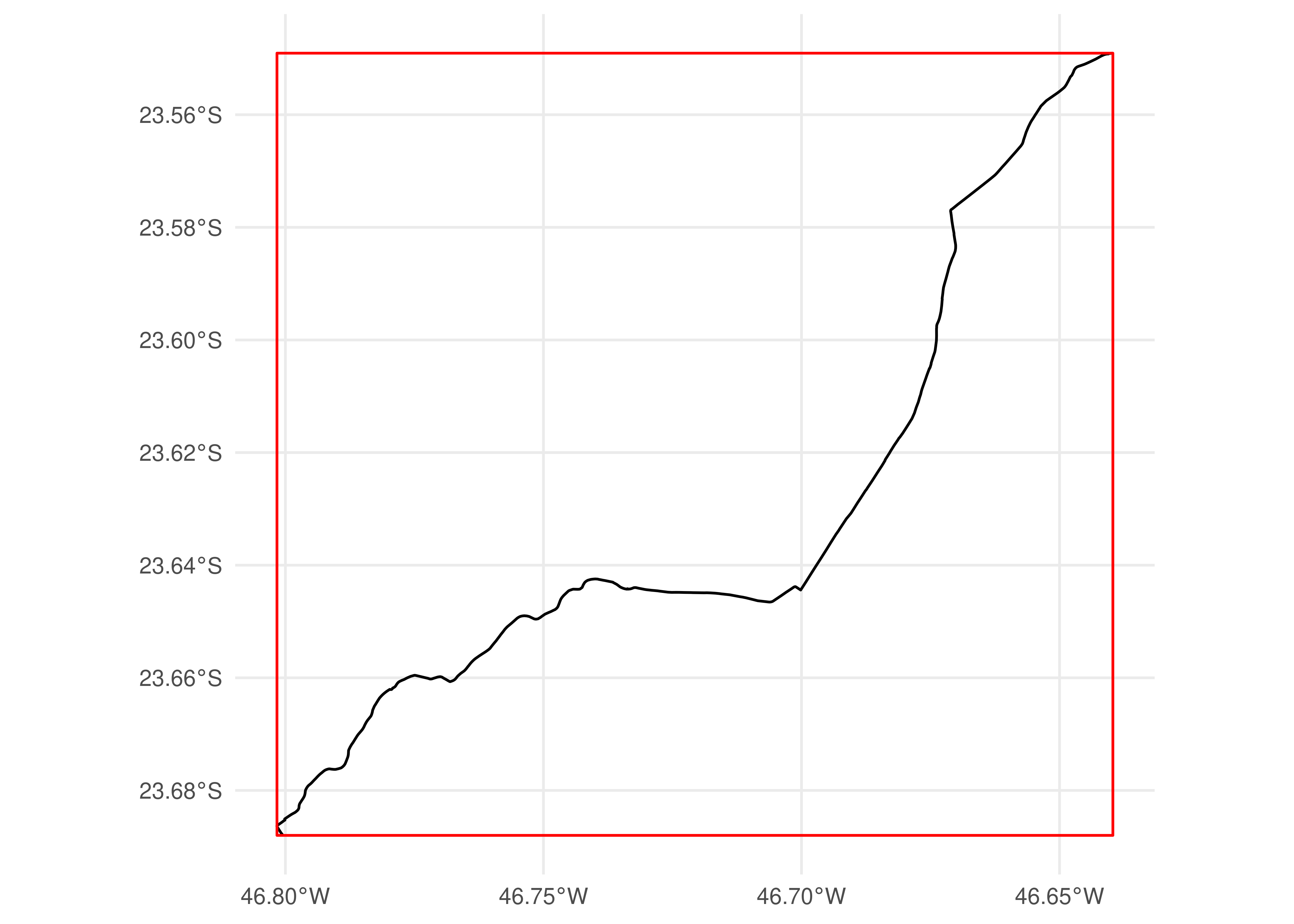
We can, however, specify different spatial operations to filter the feed. The code below shows how we can keep the entries related to trips that are contained by the specified polygon:
filtered_gtfs <-filter_by_sf(gtfs, bbox, spatial_operation = sf::st_contains)filtered_shapes <-convert_shapes_to_sf(filtered_gtfs)ggplot() +geom_sf(data = filtered_shapes) +geom_sf(data = bbox_geometry, fill =NA, color ="red") +theme_minimal()
Figure 5.3: Spatial distribution of shapes contained by the bounding box of shape 68962
5.4 Validating GTFS data
Transport planners and researchers often want to assess the quality of the GTFS data they are producing or using in their analyses. Are feeds structured following the best practices adopted by the larger GTFS community? Are tables and columns adequately formatted? Is the information described by the feed reasonable (trip speeds, stop locations, etc)? These are some of the questions that may arise when dealing with GTFS data.
To answer these and other questions, {gtfstools} includes the validate_gtfs() function. This function works as a wrapper to MobilityData’s Canonical GTFS Validator, which requires Java version 11 or higher to run2.
Using validate_gtfs() is very simple. First, we need to download the validator. To do this, we use the download_validator() function, included in the package, which receives the path to the directory where the validator should be saved to and the version of the validator that should be downloaded (defaults to the latest available). The function returns the path to the downloaded validator:
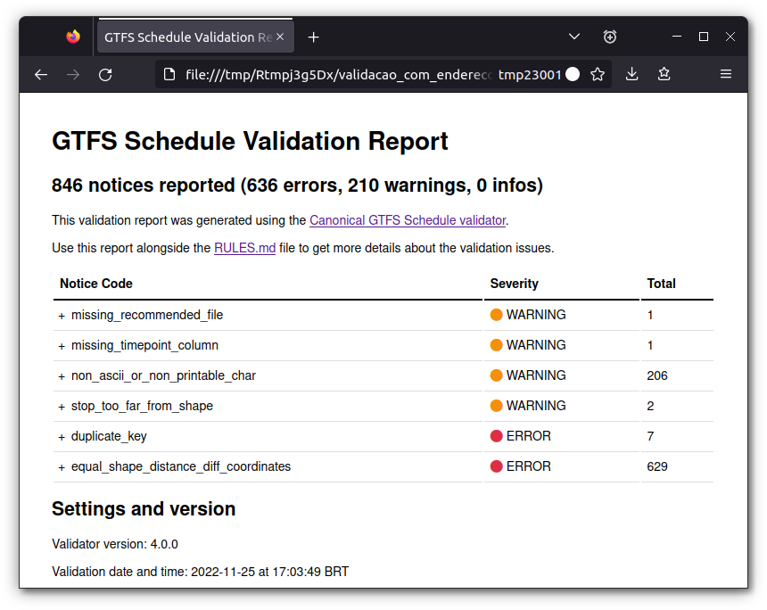
The second (and final) step consists in actually validating the GTFS data with validate_gtfs(). This function supports GTFS data in different formats: i) as a GTFS object in an R session; ii) as a path to a local GTFS file in .zip format; iii) as an URL pointing to a feed; or iv) as a directory containing unzipped GTFS tables. The function also takes a path to a directory where the validation result should be saved to and the path to the validator that should be used in the process. In the example below, we validate SPTrans’ feed from its path:
We can see that the validation process generates a few output files:
report.html, shown in Figure 5.4, which summarizes the validation result in a nicely formatted HTML page (only available with validator version 3.1.0 or higher);
report.json, which summarizes the same information, but in JSON format, which can be used to programatically parse and process the results;
system_errors.json, which summarizes eventual system errors that may have happened during the validation process and may compromise the results; and
validation_stderr.txt, which lists informative messages sent by the validator tool, including a list of the tests conducted, eventual error messages, etc3.
Figure 5.4: Validation report example
5.5{gtfstools} workflow example: spatial visualization of headways
We have shown in previous sections that {gtfstools} offers a large toolset to process and analyze GTFS files. The package, however, also includes many other functions that could not be shown in this book due to space constraints4.
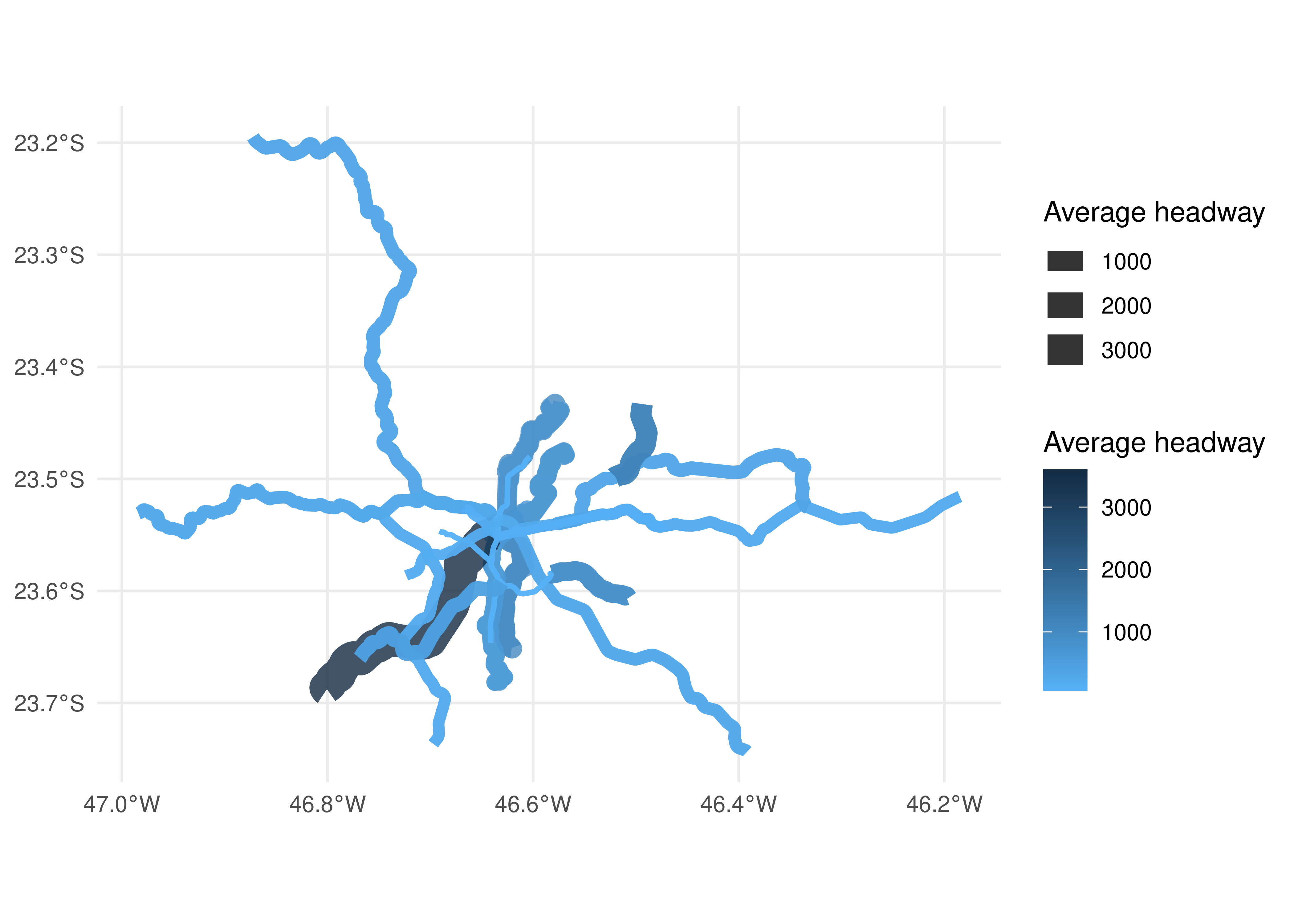
In this final section of the chapter, we illustrate how to use the package to make more complex analyses. To do this, we present a workflow that combines various functions of {gtfstools} together to answer the following question: how are the times between vehicles operating the same route (the headways) spatially distributed in SPTrans’ GTFS?
First, we need to define the scope of our analysis. In this example, we are only going to consider the services operating during the morning peak, between 7am and 9am, on a typical tuesday. Thus, we need to filter our feed:
gtfs <-read_gtfs(path)# filters the GTFSfiltered_gtfs <- gtfs |>remove_duplicates() |>filter_by_weekday("tuesday") |>filter_by_time_of_day(from ="07:00:00", to ="09:00:00")# checking the resultfiltered_gtfs$frequencies[trip_id =="2105-10-0"]
Next, we need to calculate the headways within this time interval. This information can be found at the frequencies table, though there is a factor we have to pay attention to: each trip is associated to more than one headway, as shown above (one entry for the 7am to 7:59am interval and another for the 8am to 8:59am interval). To solve this, we are going to calculate the average headway from 7am to 9am.
The first few frequencies rows in SPTrans’ feed seem to suggest that the headways are always associated to one-hour intervals, but this is neither a rule set in the official specification nor necessarily a practice adopted by other feed producers. Thus, we have to calculate the average headways weighted by the time duration of each headway. To do this, we need to multiply each headway by the size of the time interval during which it is valid, sum these multiplication results for each trip, and then divide this amount by the total time interval (two hours, in our case). To calculate the time intervals within which the headways are valid, we first use the convert_time_to_seconds() function to calculate the start and end time of the time interval in seconds and then subtract the latter by the former:
filtered_gtfs <-convert_time_to_seconds(filtered_gtfs)# check how the results look like for a particular trip idfiltered_gtfs$frequencies[trip_id =="2105-10-0"]
Now we need to generate each trip geometry and join this data to the average headways. To do this, we will use the get_trip_geometry() function, which returns the spatial geometries of the trips in the feed. This function allows us to specify which trips we want to generate the geometries of, so we are only going to apply the procedure to the trips present in the average headways table:
Finally, we need to join the average headway data to the geometries and then configure the map as wished. In the example below, the color and line width of each trip geometry varies with its headway:
Figure 5.5: Headways spatial distribution in SPTrans’ GTFS
As we can see, {gtfstools} makes the analysis of GTFS feeds a simple task that requires only basic knowledge of table manipulation packages (such as {data.table} or {dplyr}). The example shown in this section illustrates how one could use many of the package’s functions together to reveal important aspects of public transport systems specified in the GTFS format.
For more information on how to check the installed version of Java in your computer and on how to install the required version, please check Chapter 3.↩︎
Informative messages may also be listed in the validation_stdout.txt file. Whether messages are listed in this file or in validation_stderr.txt depends on the validator version.↩︎