Introduction to urban accessibility: a practical guide with R

Rafael H. M. Pereira; Daniel Herszenhut

doi:http://dx.doi.org/10.38116/9786556350547

8 Data on the spatial distribution of opportunities

The {aopdata} package allows one to download data from 2017, 2018 and 2019 on the spatial distribution of jobs (low, middle and high education), public health facilities (low, medium and high complexity), public schools (early childhood, primary and secondary school levels) and CRAS. This data is available for all cities included in the project.

These datasets can be downloaded with the read_landuse() function, which works similarly to read_population(). To use it, indicate the city whose data should be downloaded using the city parameter, along with the reference year (year) and whether to include the spatial information of grid cells or not (geometry).

In the example below, we show how to download land use data from 2019 for the city of Belo Horizonte. Please note that this function outputs a table that also includes sociodemographic data.

data_bh <- aopdata::read_landuse(
  city = "Belo Horizonte",
  year = 2019,
  geometry = TRUE,
  showProgress = FALSE
)

names(data_bh)

 [1] "id_hex"      "abbrev_muni" "name_muni"   "code_muni"   "P001"       
 [6] "P002"        "P003"        "P004"        "P005"        "P006"       
[11] "P007"        "P010"        "P011"        "P012"        "P013"       
[16] "P014"        "P015"        "P016"        "R001"        "R002"       
[21] "R003"        "year"        "T001"        "T002"        "T003"       
[26] "T004"        "E001"        "E002"        "E003"        "E004"       
[31] "M001"        "M002"        "M003"        "M004"        "S001"       
[36] "S002"        "S003"        "S004"        "C001"        "geometry"

Table 8.1 presents the data dictionary with the description of the table columns (excluding those previously included in the sociodemographic dataset). This description can also be found in the documentation of the function, running the command ?read_landuse in an R session.

Table 8.1: Description of the columns in the land use dataset
Column	Description
year	Reference year
id_hex	Unique hexagon identifier
abbrev_muni	3-letter abbreviation of municipality name
name_muni	Municipality name
code_muni	7-digit municipality IBGE code
T001	Total number of jobs
T002	Number of low-education jobs
T003	Number of middle-education jobs
T004	Number of high-education jobs
E001	Total number of public schools
E002	Number of public early childhood schools
E003	Number of public primary schools
E004	Number of public secondary schools
M001	Total number of students enrolled in public schools
M002	Number of students enrolled in public early childhood schools
M003	Number of students enrolled in public primary schools
M004	Number of students enrolled in public secondary schools
S001	Total number of public health facilities
S002	Number of low complexity public health facilities
S003	Number of mid complexity public health facilities
S004	Number of high complexity public health facilities
C001	Total number of CRAS
geometry	Spatial geometry

The following sections show a few examples illustrating how to create spatial visualizations out of this dataset.

8.1 Spatial distribution of jobs

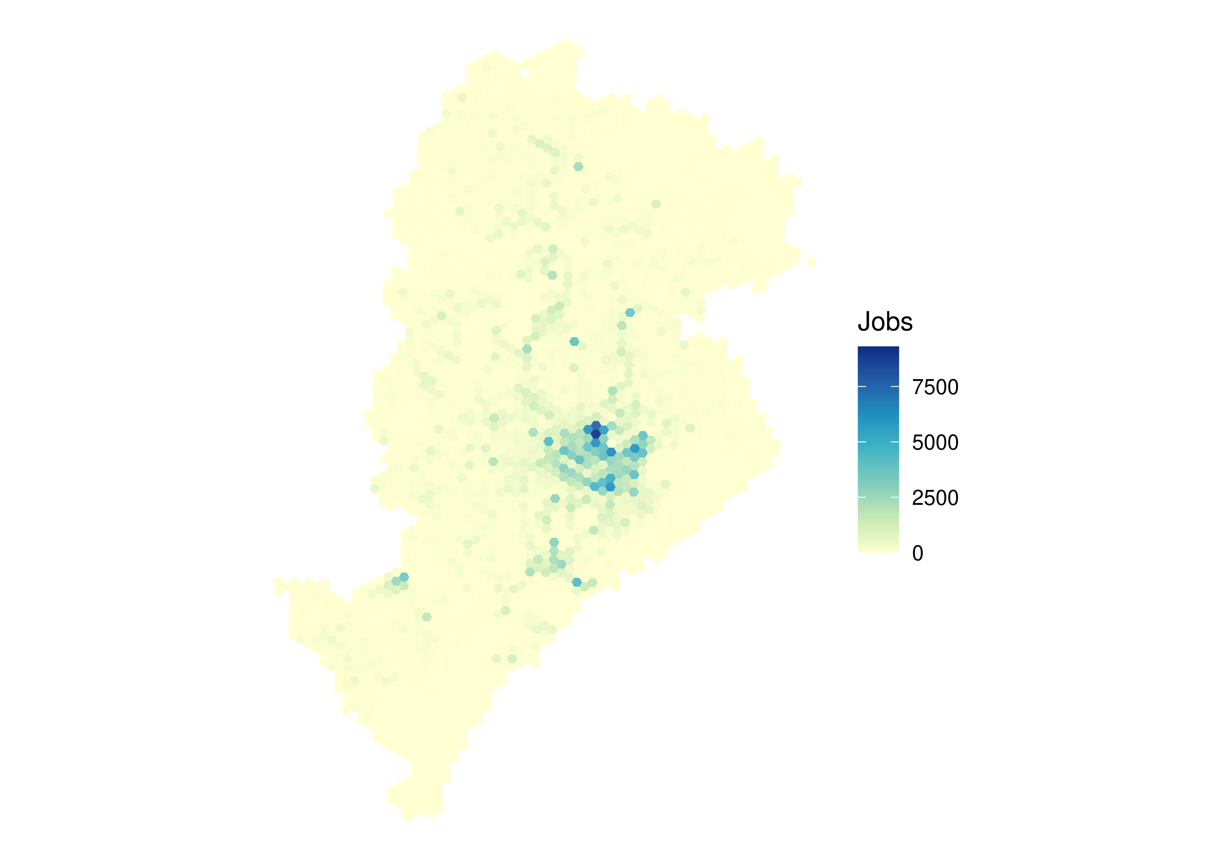
In the code below, we load a couple data visualization libraries and configure the map. Columns starting with the letter T describe the spatial distribution of jobs in each city. The example shows the spatial distribution of the total number of jobs in each grid cell (variable T001) in Belo Horizonte:

library(patchwork)
library(ggplot2)

ggplot(data_bh) +
  geom_sf(aes(fill = T001), color = NA, alpha = 0.9) +
  scale_fill_distiller(palette = "YlGnBu", direction = 1) +
  labs(fill = "Jobs") +
  theme_void()

Figure 8.1: Spatial distribution of jobs in Belo Horizonte

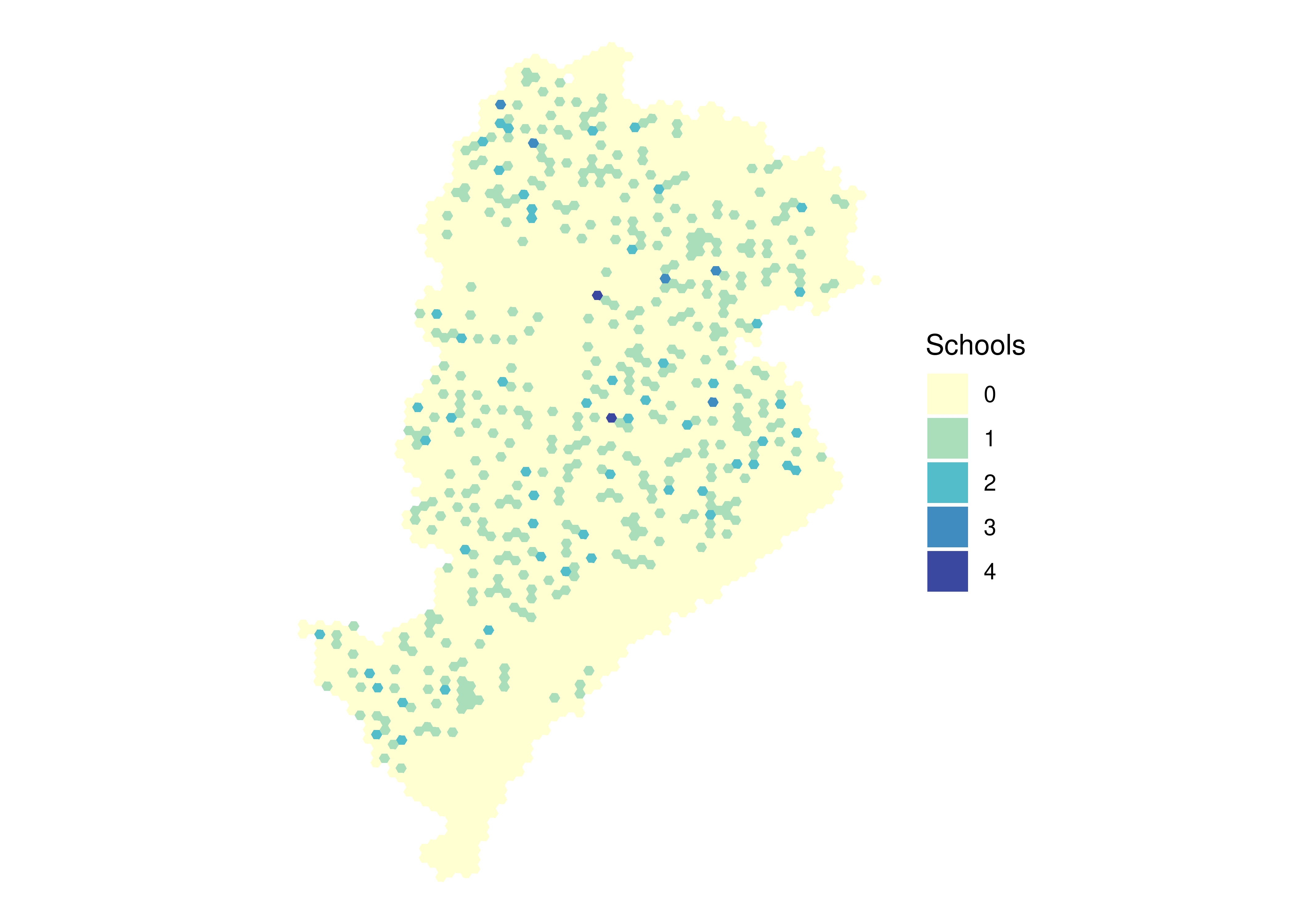
8.2 Spatial distribution of public schools

The columns with information on the number of public schools in each cell begin with the letter E. In the example below, we present the spatial distribution of all public schools in Belo Horizonte (variable E001).

ggplot(data_bh) +
  geom_sf(aes(fill = as.factor(E001)), color = NA, alpha = 0.9) +
  scale_fill_brewer(palette = "YlGnBu", direction = 1) +
  labs(fill = "Schools") +
  theme_void()

Figure 8.2: Spatial distribution of public schools in Belo Horizonte

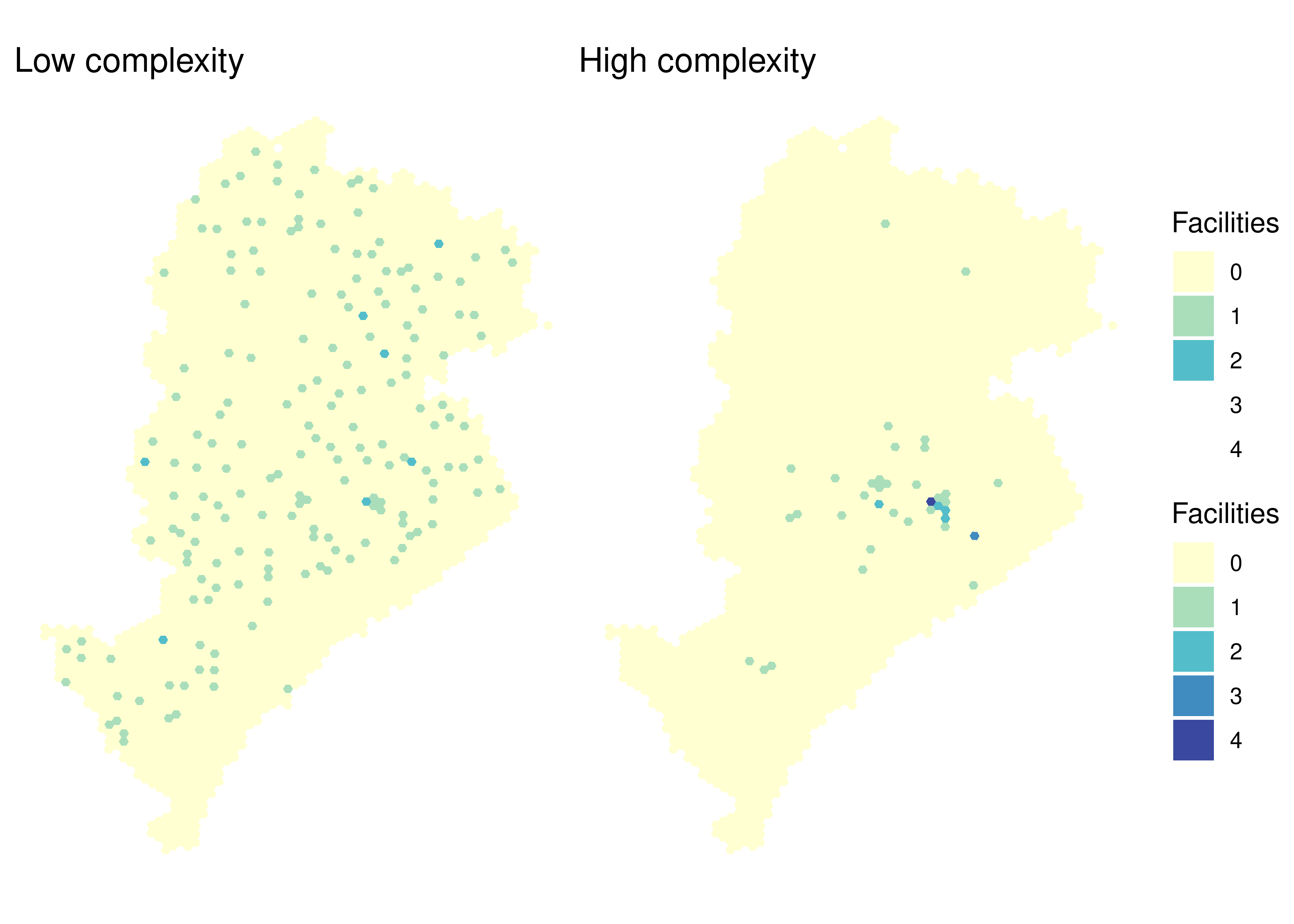
8.3 Spatial distribution of public health facilities

The columns with information on the number of public health facilities in each cell begin with the letter S. The visualization below compares the spatial distribution of low complexity (S002) and high complexity (S004) public health facilities.

low_complexity <- ggplot(data_bh) +
  geom_sf(aes(fill = as.factor(S002)), color = NA, alpha = 0.9) +
  scale_fill_brewer(palette = "YlGnBu", direction = 1, limits = factor(0:4)) +
  labs(title = "Low complexity", fill = "Facilities") +
  theme_void()

high_complexity <- ggplot(data_bh) +
  geom_sf(aes(fill = as.factor(S004)), color = NA, alpha = 0.9) +
  scale_fill_brewer(palette = "YlGnBu", direction = 1, limits = factor(0:4)) +
  labs(title = "High complexity", fill = "Facilities") +
  theme_void()

low_complexity + high_complexity + plot_layout(guides = "collect")

Figure 8.3: Spatial distribution of low complexity and high complexity public health facilities in Belo Horizonte

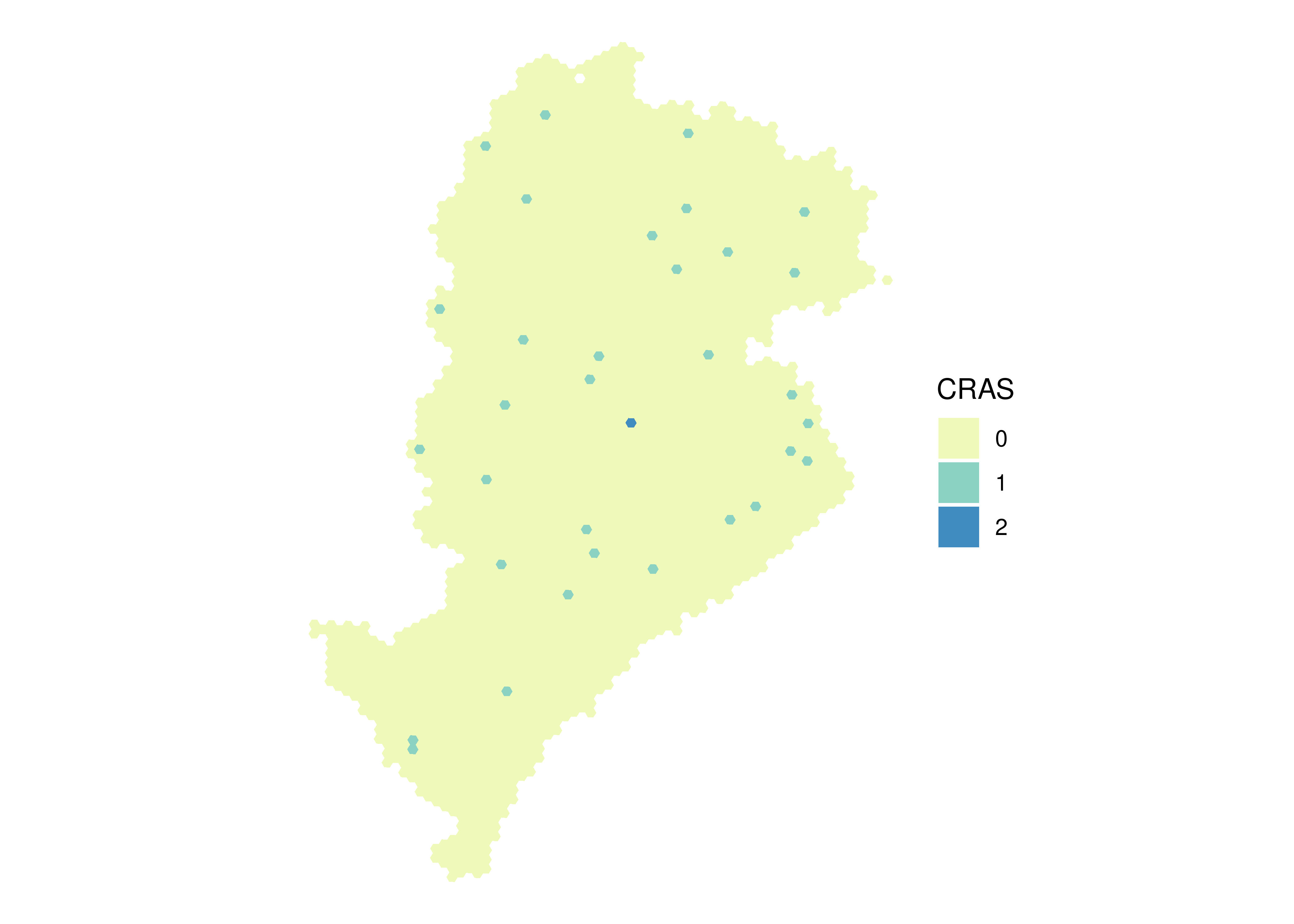
8.4 Spatial distribution of CRAS

Finally, the column C001 has information on the number of CRAS in each grid cell. The map below shows the spatial distribution of these services in Belo Horizonte.

ggplot(data_bh) +
  geom_sf(aes(fill = as.factor(C001)), color = NA, alpha = 0.9) +
  scale_fill_brewer(palette = "YlGnBu", direction = 1) +
  labs(fill = "CRAS") +
  theme_void()

Figure 8.4: Spatial distribution of CRAS in Belo Horizonte